HS-3000: Fit Method Comparison - Approximation on the Arm Model
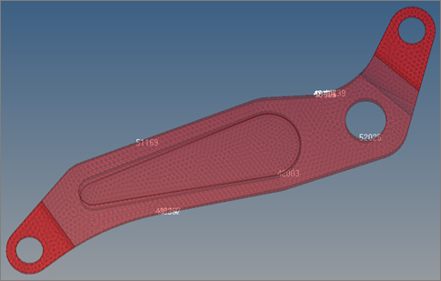
Tutorial Level: Intermediate Learn how to create approximations for the output responses of the arm example introduced in tutorial, and review the differences between different Fit methods.
In HS-2000: DOE Method Comparison: Arm Model Study, you learned that instead of using the nine input variables, you could continue additional studies just as effectively with six shapes since the others did not have a great influence on the output responses. This will save computational effort.
- Length1: Lower Bound = -0.5, Initial Bound = 0.0, Upper Bound = 2.0
- Length2: Lower Bound = 0.0, Initial Bound = 0.0, Upper Bound = 2.0
- Length3: Lower Bound = -1.0, Initial Bound = 0.0, Upper Bound = 1.0
- Length4: Lower Bound = -1.0, Initial Bound = 0.0, Upper Bound = 1.0
- Length5: Lower Bound = -1.0, Initial Bound = 0.0, Upper Bound = 1.0
- Height: Lower Bound = -1.0, Initial Bound = 0.0, Upper Bound = 1.0
Run MELS DOE Study
In this step you will create a Modified Extensible Lattice Sequence (MELS) DOE. You will use this matrix to create the Fits for both output responses.
MELS is a space filling DOE designed to equally spread out points in a space by minimizing clumps and empty spaces. The minimal required number of points to create a second order polynomial with N variables is 1.1*(N + 1)*(N + 2)/2.
In order to create the approximations to be used as surrogate models, you must perform specific DOEs that will serve as the input matrix. You will need to run a DOE suitable to be used in response surface creation, such as MELS.
-
Add a DOE.
-
Modify input variables.
- Go to the step.
- In the work area, Active column, clear the radius_1, radius_2, and radius_3 checkboxes.
Figure 1. 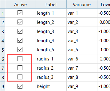
-
Define specifications.
- Go to the step.
- In the work area, set the Mode to Modified Extensible Lattice Sequence (MELS).
- In the Settings tab, verify that the Number of Runs is set to 31.
- Click Apply.
-
Evaluate tasks.
- Go to the step.
- Click Evaluate Tasks.
- Go to the step.
-
Click the Scatter tab to review a 2D scatter plot of the results from the MELS
DOE.
Figure 2. Typical Sampling of the MELS DOE with 31 Runs (length_1 vs. length_2). This visualization is a projection of 31 points distributed in 6 dimensions onto a 2 dimensional plane. 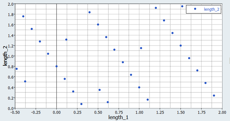
Optional: Run DOE with Less Runs
In this step you will create an optional second DOE with less number of runs to be used as a Validation matrix in the Fit approach.
In this tutorial, you will use the Hammersley method to create the Validation matrix.
-
Add a DOE.
-
Define specifications.
-
In the Settings tab, change the Number of Runs to
12.
Figure 3. 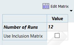
-
In the Settings tab, change the Number of Runs to
12.
-
Evaluate tasks.
- Go to the step.
- Click Evaluate Tasks.
Run Fits
In this step you will use the 31 runs from the MELS DOE as an Input matrix and the 12 runs from the Hammersley DOE as a Validation matrix to create four Fits using Least Square Regression (LSR), Moving Least Square Method (MLSM), HyperKriging (HK), and Radial Basis Function (RBF).
-
Add a Fit.
- In the Study Explorer, right-click and select Add from the context menu.
- In the Add dialog, select Fit Existing Data and Setup, and click OK.
-
Import matrix.
- Go to the step.
- Click Add Matrix twice.
- In the work area, define Fit Matrix 1 and Fit Matrix 2 by selecting the options indicated in Figure 4.
- Click Apply.
Figure 4. 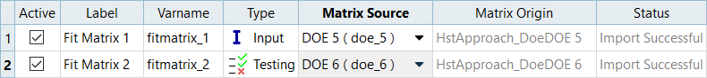
-
Define specifications.
-
In the work area, Fit Type column, select the appropriate Fit
method.
Important:
For the Least Square Regressions (LSR) Fit, in the Settings tab, set Regression Model to Interaction.
An Interaction regression model enables linear and cross terms to be considered in the function f(x,y)=A+Bx+Cy+Dxy; where the first three terms are linear, and the last term is a cross term between the variables.
Figure 5. 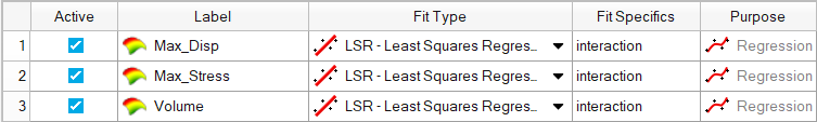
-
In the work area, Fit Type column, select the appropriate Fit
method.
-
Evaluate tasks.
- Go to the step.
- Click Evaluate Tasks.
- Go to the step.
-
Click the Scatter tab to compare the original Max_Stress
output response to the Fit Max_Stress.
The scatter shows the Fit accuracy. The closer together the points are along the diagonal, the better the fit. In the Max_Stress vs Max_Stress_LSR plot, you can see some dispersed points, which indicates the Fit has some inaccuracy. In comparison, the points in the Max_Stress vs Max_Stress_MLSM plot follow the diagonal more closely, which indicates it provides better Fit accuracy on Max_Stress.
You will not compare HyperKriging and Radial Basis Function using scatter plots, because the results will be misleading. HyperKriging and Radial Basis Function go through the exact points by default, therefore the scatter plot comparing the original output response vs. the Fit output response will produce a straight line. However, this does not necessarily mean that the Fit has good predictive capability.Figure 6. Max_stress and Max_stress, LSR Comparison 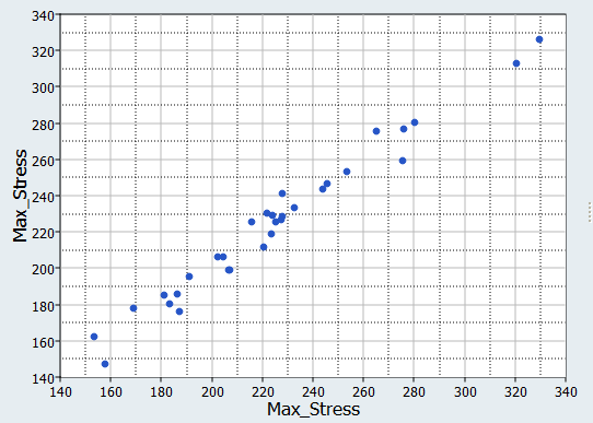
Figure 7. Max_stress and Max_stress, MLSM Comparison 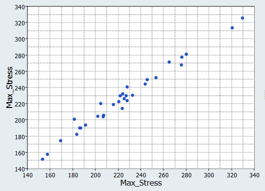
-
Click the Diagnostics tab to review the diagnostics of
the Fit study.
The R-Square value measures how much of the variability of the response data around its mean is captured. If the model perfectly predicts the known values, R-Square will have a maximum possible value of 1.0.
Figure 8. Diagnostics for Max_Stress, LSR 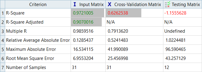
Figure 9. Diagnostics for Max_Stress, MLSM 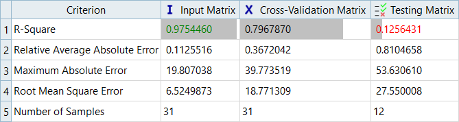
The R-square value for an Input Matrix in HyperKriging and Radial Basis Function has no meaning because the runs will always go through the exact data points, which will result in a value of 1.0. Although the value is 1.0, this does not mean the Fit will be accurate. In HyperKriging and Radial Basis Function, the only meaningful diagnostic values are for Cross-validation Matrix and Validation Matrix.Figure 10. Diagnostics for Max_Stress, HK 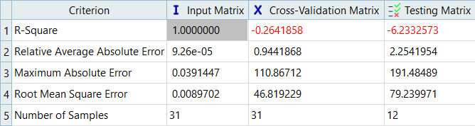
Figure 11. Diagnostics for Max_Stress, RBF 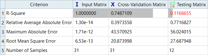
-
Click the Residuals tab to review the Error (and Percent
Error) between the original output response and the Fit output response for each
run of the Input and Testing matrices.
Figure 12. Input Matrix Residuals on Max_Stress, LSR 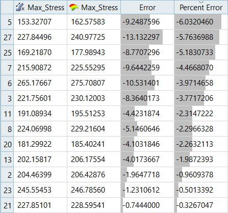
Figure 13. Testing Matrix Residuals on Max_Stress, LSR 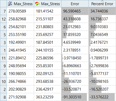
The Input Matrix Residual errors are slightly smaller with Least Square Regression, than they are with Moving Least Square Method, but the Testing Matrix Residual errors are much smaller with Moving Least Square Method.Figure 14. Input Matrix Residuals on Max_Stress, MLSM 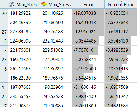
Figure 15. Testing Matrix Residuals on Max_Stress, MLSM 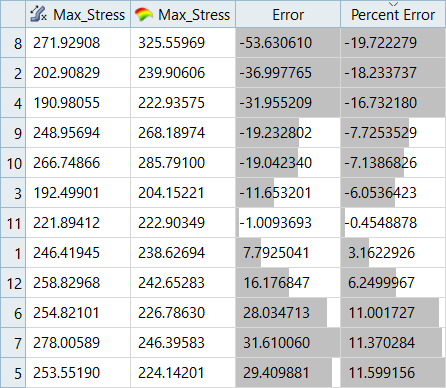
The Input Matrix Residuals are meaningless for HyperKriging and Radial Basis Function, as indicated in the Testing Matrix Residuals below.Figure 16. Testing Matrix Residuals on Max_Stress, HK 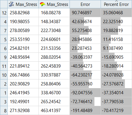
Figure 17. Testing Matrix Residuals on Max_Stress, RBF 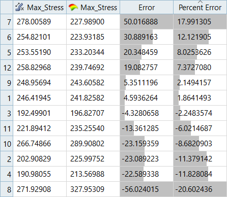
Fit Comparison
Overview of the max percent of errors for Input and Testing matrices.
| LSR (Interaction Regression Model) | MLSM | HK | RBF | |
|---|---|---|---|---|
| Max_Disp | -1.18% | -2.79% | - | - |
| Max_Stress | -6.72% | -10.92% | - | - |
| LSR (Interaction Regression Model) | MLSM | HK | RBF | |
|---|---|---|---|---|
| Max_Disp | 7.26% | -3.00% | 9.57% | -2.45% |
| Max_Stress | 34.74% | -19.72% | 35.06% | 17.99% |
It can be seen that the percent of errors for Max_Disp are smaller than Max_Stress. These results indicate the Fit approach works well for Max_Disp, but is not very efficient for Max_Stress.