
Plot Run Time Data
Use the Plot tool to track converged and derived solution behavior in real time.
- Select the Plot icon on the Solution ribbon.
Figure 1. 
- From the Run Status dialog, right-click on an AcuSolve run and select Plot time history from the context menu.
If AcuSolve is still running, the plots update in real time to track the solution progress.
Create Plots
Select data of interest to plot and then add it to a preview plot. Once all curves are added to the preview plot, the plot is available for placement on the plotting canvas.
-
In the Plot Manager, click
 to create a new plot.
- Optional:
Click
 to import an existing plot definition.
This allows you to read results data from multiple AcuSolve runs at once and use them as data sources for your plats.
to import an existing plot definition.
This allows you to read results data from multiple AcuSolve runs at once and use them as data sources for your plats. -
Define the y-axis.
Figure 3. 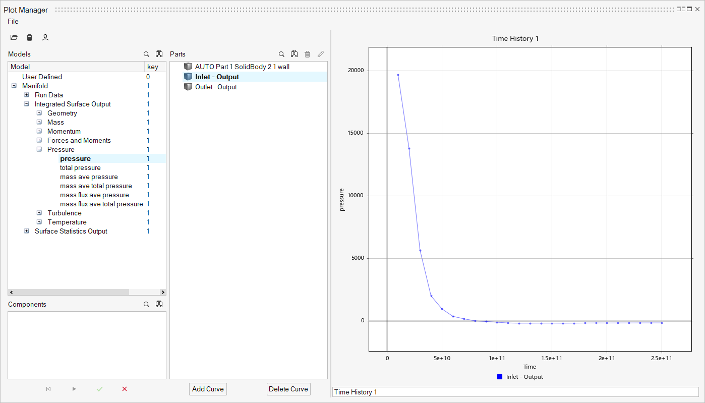
- Optional: Click the x-axis to cycle between values.
- Optional: Change the name of the plot using the text box below the preview.
- Click Add Curve to add your plot to the preview.
-
Select one of the following:
 - Plot previewed curves and continue creating
plots.
- Plot previewed curves and continue creating
plots. - Plot previewed curves and return to the base
view.
- Plot previewed curves and return to the base
view. - Delete preview and return to the base view.
 - Clear the preview.
Plot User Defined Functions
Use a python-based scripting language to define new functions from existing curve data.
-
In the Plot Manager, click to create a new plot.
-
Do one of the following:
- Click
 .
. - Right-click on User Defined in the Model Pane and select Create New.
- Click
- Enter a name for the function.
-
Enter a python script in terms of "Get", "time", "step", or "value".
For example:
cpu = runData(1.'Run Data'.'CPU Time')
elapsed = runData(1.'Run Data'.'Elapsed Time')
value = cpu/elapsedor
value = 1 + step
-
Select data types, components, and parts to add to the function if
needed.
Note: Click
 to insert the field into the UDF editor with
the correct syntax.
to insert the field into the UDF editor with
the correct syntax. -
Select one of the following:
- - Add the function to the plot
preview.
 - Save the function.
-
- Delete the function.
Tip: Click to edit a UDF.
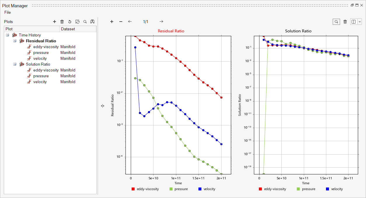
Edit the Plotting Canvas
The canvas layout can be changed to accommodate more plots on a given page. Additional pages can also be created.
-
In the base view of the Plot Manager, click or
 to add/delete pages then use the arrows to cycle between them.
- Use the drop-down on the far right to change the layout of the page and allow for more or less plots.
-
Double-click on an empty plot to select it, then right-click on a data set and
select Make Current to plot it.
You can also edit, rename, delete, and export by right-clicking on data sets and variables.
-
Scroll to zoom in or out on a plot and right-click and drag to pan.
Click
 to return to a fitted view.
 - To edit display properties, right-click on a curve, plot, or variable.