
Turbulent Flow Through a Heated Periodic Channel
In this application, AcuSolve is used to solve for the flow and temperature field within a channel containing a heated wall. The wall is maintained at a constant temperature, inducing heat flux into the fluid, to predict the thermal law of the wall. The non-dimensional temperature versus the non-dimensional height above the wall is compared to the analytical correlation provided by Kader.
Problem Description
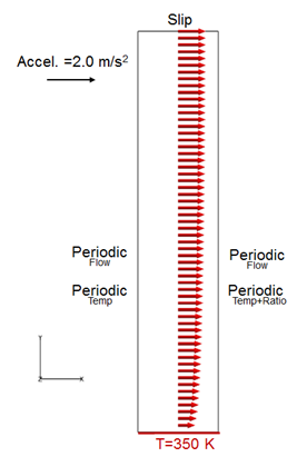
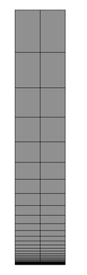
The simulation was performed as a two-dimensional problem by constructing a volume mesh that contains a single layer of elements extruded in the cross-stream direction, normal to the flow plane and by imposing periodic boundary conditions on the extruded planes. The streamwise direction contains two elements allowing the flow and temperature solution to develop. Only the lower half of the channel is modeled, assuming the solution is mirror across the top slip plane.
AcuSolve Results
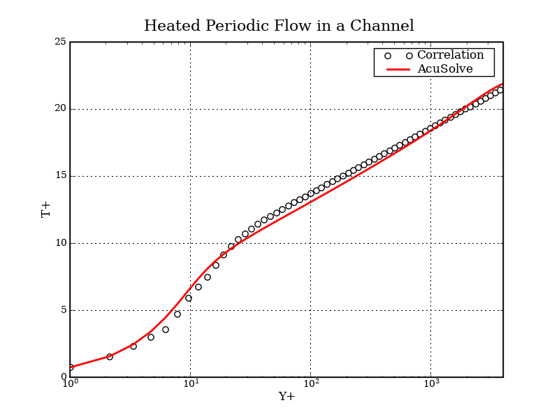
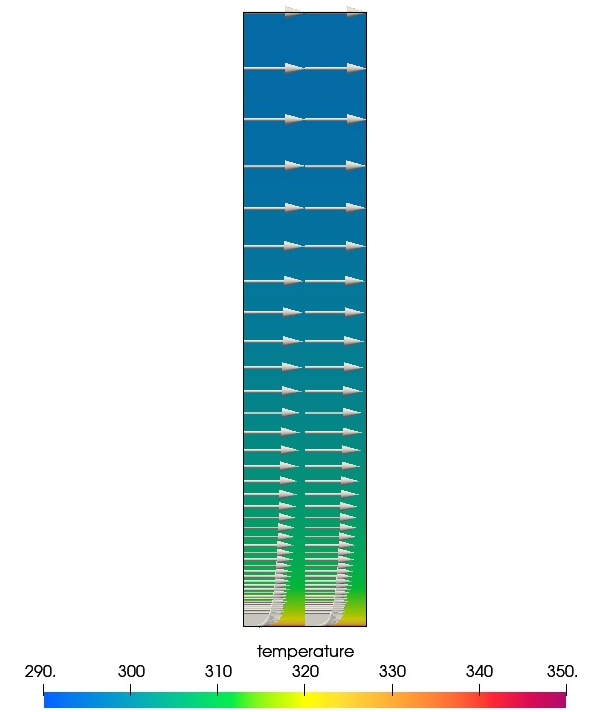
The AcuSolve solution converged to a steady state and the results reflect the mean flow conditions within the channel. The simulation results demonstrate that the channel wall induces a thermal flux into the flow field, producing a temperature distribution dependent on the distance from the wall. The thermal law of the wall computed from the AcuSolve results is compared with correlation data for the corresponding Prandtl number, as demonstrated in Kader 1981. The plot shown below gives the non-dimensional value of T+ as a function of Y+, where T+ and Y+ are computed per the following relationships:
Where , is the fixed wall temperature, T is the temperature away from the wall, is the fluid density, is the fluid specific heat, is computed from the magnitude of the shear stress and is the local surface heat flux.
Summary
The AcuSolve solution compares well with the correlation data for turbulent flow within a heated channel. In this application, the constant temperature wall induces a surface heat flux, giving rise to a temperature gradient within the channel. AcuSolve can capture the correct temperature gradient at any location above the wall if an appropriate first layer height is selected to resolve a Y+ value of 1.0. The good agreement with correlation data for T+ demonstrates that AcuSolve can predict the locally varying temperature distribution within a turbulent channel.
Simulation Settings for Turbulent Flow Through a Heated Periodic Channel
SimLab database file: <your working directory>\channel_periodic_heat\channel_periodic_heat.slb
Global
- Problem Description
- Flow type - Steady State
- Temperature equation - Advective Diffusive
- Turbulence equation - Spalart Allmaras
- Auto Solution Strategy
- Max time steps - 50
- Convergence tolerance - 0.0001
- Relaxation Factor - 0.4
- Temperature - On
- Material Model
- Fluid
- Type - Constant
- Density - 1.0 kg/m3
- Viscosity - 1.0e-4 kg/m*sec
- Specific Heat - 1005.0 J/kg*K
- Conductivity - 0.139 W/m*K
- Fluid
- Body Force
- BodyForce
- Gravity
- X-component - 2.0 m/sec2
- Gravity
Model
- BodyForce
- Volumes
- Fluid
- Element Set
- Material model - Fluid
- Body force - BodyForce
- Element Set
- Fluid
- Surfaces
- Symmetry_1
- Simple Boundary Condition - (disabled to allow for periodic conditions to be set)
- Symmetry_2
- Simple Boundary Condition - (disabled to allow for periodic conditions to be set)
- Inflow
- Simple Boundary Condition - (combination of integrated BC and periodic BC set)
- Advanced Options
- Integrated Boundary Conditions - Temperature - 300.0 K
- Outflow
- Simple Boundary Condition - (disabled to allow for periodic conditions to be set)
- Slip_surface
- Simple Boundary Condition
- Type- Slip
- Simple Boundary Condition
- Wall_surface
- Simple Boundary Condition
- Type- Wall
- Temperature BC type - Value
- Temperature - 350.0 K
- Simple Boundary Condition
- Symmetry_1
- Periodics
- 2D
- Periodic Boundary Conditions
- Type - Periodic
- Periodic Boundary Conditions
- Flow
- Periodic Boundary Conditions
- Type - Periodic
- Periodic Boundary Conditions
- Temperature
- Individual Periodic BCs
- Temperature: Type - Single Unknown Ratio
- Individual Periodic BCs
- 2D
- Nodes
- Zero_z-velocity
- Z-Velocity: Type - Zero
- Zero_z-velocity
References
B.A. Kader, "Temperature and concentration profiles in fully turbulent boundary layers", International Journal of Heat and Mass Transfer, Volume 24, Issue 9, 1981, Pages 1541-1544.
H. Kawamura, K. Ohsaka, H. Abe and K. Yamamoto, "DNS of turbulent heat transfer in channel flow with low to medium-high Prandtl number fluid", International Journal of Heat and Mass Transfer, 19:482-491, 1998.