Laminar Couette Flow with Imposed Pressure Gradient
In this application, AcuSolve is used to simulate the
viscous flow of water between a moving and a stationary plate with an imposed pressure
gradient. AcuSolve results are compared with analytical results
described in White (1991). The close agreement of AcuSolve
results with analytical results validates the ability of AcuSolve to model cases with imposed pressure gradients.
Problem Description
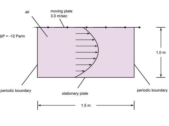
The problem consists of air between two plates in a two dimensional domain, as shown in the
following image, which is not drawn to scale. The domain is 1.0 m high and 1.5 m
long. The top plate moves with a constant velocity of 3.0 m/sec and the bottom plate
is fixed. There is a mean-pressure gradient of -12 Pa/m applied to the bulk fluid in
the streamwise direction. The problem is simulated with periodic boundaries in the
streamwise direction. The induced flow field is laminar and exhibits a steady state
behavior. The flow field develops from the pressure gradient, the motion of the top
plate, and the viscous shear stresses near the plates.Figure 1. Critical Dimensions and Parameters for Simulating Laminar Couette Flow
with an Imposed Pressure Gradient
The simulation was performed as a two dimensional problem by restricting flow in the out-of-plane
direction through the use of a mesh that is one element thick.Figure 2. Mesh used for Simulating Laminar Couette Flow with an Imposed Pressure
Gradient
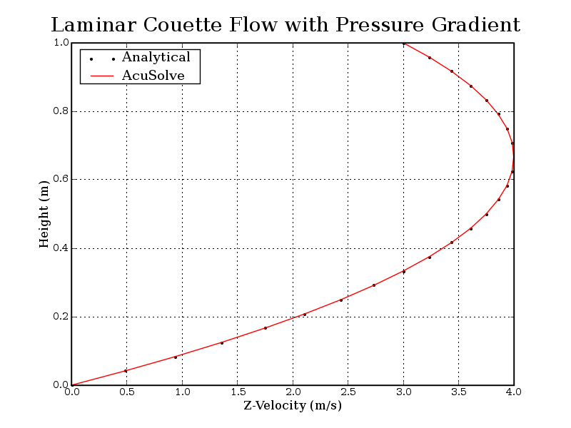
AcuSolve Results
The AcuSolve solution converged to a steady state and the results
reflect the mean flow conditions. The greatest velocity is located at approximately
40 percent of the channel height, closer to the moving plate. The flow develops as a
result of the pressure gradient and the shear stress acting on the fluid near both
the moving plate and the stationary plate.Figure 3. Z-Velocity Contours and Velocity Vectors Figure 4. Z Velocity Plotted Against Height Above the Bottom of the Flow Field (Z
Velocity is Presented on the X Axis to Better Represent the Velocity Profile
in the Direction of Flow)
Summary
The velocity profile computed by AcuSolve agrees well with the
analytical solution for this application. The velocity profile arises due to the
combination of the imposed pressure gradient and the constant upper-wall velocity.
Note: The combination of these effects results in the asymmetric velocity
profile that is reflected in the results.
Simulation Settings for Laminar Couette Flow with Imposed Pressure Gradient
SimLab database file: <your working
directory>\couette_flow\couette_flow.slb
Global
Problem Description
Solution Type - Steady State
Flow - Laminar
Auto Solution Strategy
Relaxation factor - 0.2
Material Model
Air
Density - 1.0 kg/m3
Viscosity - 1.0 kg/m-sec
Body Force
DP/DL
Gravity
Z-component - 18.0 m/sec2
Model
Volumes
Fluid
Element set
Material model - Air
Body force - DP/DL
Surfaces
Max_X
Simple Boundary Condition
Type - Symmetry
Max_Y
Simple Boundary Condition
Type - Wall
Wall velocity type - Cartesian
Z-velocity - 3.0 m/s
Max_Z
Simple Boundary Condition - (disabled to allow for periodic
conditions to be set)
Min_X
Simple Boundary Condition
Type - Symmetry
Min_Y
Simple Boundary Condition
Type - Wall
Min_Z
Simple Boundary Condition - (disabled to allow for periodic
conditions to be set)
Periodics
Periodic 1
Periodic Boundary Conditions
Type - Periodic
References
F. M. White. “Viscous Fluid Flow”. Section 3-2.3. McGraw-Hill Book Co., Inc.
New York. 1991.