Since version 2026, Flux 3D and Flux PEEC are no longer available.
Please use SimLab to create a new 3D project or to import an existing Flux 3D project.
Please use SimLab to create a new PEEC project (not possible to import an existing Flux PEEC project).
/!\ Documentation updates are in progress – some mentions of 3D may still appear.
How can I speed up my solving?
In order to speed up computation times, Flux offers its users the ability to parallelize and do some parametric distribution for heavy project computations.
Solver parallelization
During finite element solving, several steps may be achieved in parallel (using several cores available on the machine) such as the building of the topological matrix, the assembly, and the solving of the linear system, which usually is the most time-consuming task.
All the steps described above directly depend on the number of nodes in the Flux project mesh. An optimal number of cores usually exists and allows to divide of the computations among the different cores without spending too much time on the synchronization between them. This optimal number of cores reduces the calculation times as much as possible, without overloading the machine used.
This document uses 2D, 3D, and Skew examples to give recommendations in terms of number of cores, linear solver, and an estimation of the memory needed. To do this, a case has been selected for each application (Transient Magnetic, Steady-State AC magnetic, and Magnetostatic). This case is solved several times with a different mesh, a different number of cores, from 1 to 32, and different solvers (direct or iterative).
Parametric Distribution
The parametric distributed computing allows the user to save computation time while distributing several independent configurations of the same Flux project. For example, a Magnetic Transient project may be distributed regarding different values of parameters such as the geometrical parameters (size, shape, etc...) or physical parameters (supply current values, speed...) varying in the scenario. Several projects will run at the same time simulating all those configurations, the main parameter of a distributed computation is the number of running Flux in parallel.
This document shows the establishment of a parametric distribution on a single machine and a cluster. For the single-machine distribution, an internal tool of Flux is employed while PBS and other schedulers may be used on a cluster.
Recommendations to speed up your solving
From a simple 2D case to a full 3D model representing a complex electromagnetic device, the finite element problems may be drastically different and do not always require the same needs in terms of computation resources.
- Should I use parametric distribution to decrease solving time?
- Should I use solver parallelization to decrease solving time?
This document orients the user to find the best way to decrease efficiently its computation time.
The best linear solver is Automatic, as it automatically chooses to use the Direct or Iterative solver, depending on the application type and the number of nodes in the mesh.
| Mesh size | Number of parameters in the scenario | Use of parametric distribution | Use of solver parallelization | |
|---|---|---|---|---|
| Flux 2D | 0-100k | 0-10 | No | No |
| 0-100k | 10 + | Yes, single machine or cluster | No | |
| 100k + | 0-10 | No | Yes, see the recommendations | |
| 100k + | 10 + | Yes, single machine or cluster | Yes, see the recommendations |
| Mesh size (extruded geometry) |
Use of solver parallelization | |
|---|---|---|
| Flux Skew | 0-300k | No |
| 300k + | Yes, see the recommendations |
| Mesh size | Number of parameters in the scenario | Use of parametric distribution | Use of solver parallelization | |
|---|---|---|---|---|
| Flux 3D | 0-75k | 0-10 | No | No |
| 0-75k | 10+ | Yes, single machine or cluster | No | |
| 75k + | 0-10 | No | Yes, see the recommendations | |
| 75k + | 10+ | Yes, single machine or cluster | Yes, see the recommendations |
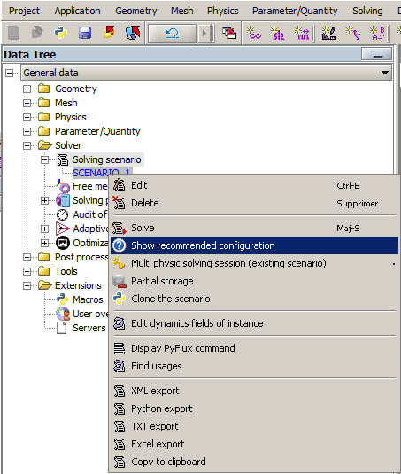
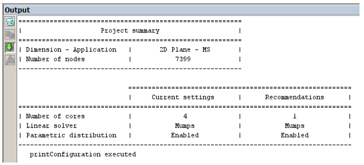
To help you, you can use the recommended configurations given by Flux. There are displayed when you create a new scenario, when you click on Show recommended configuration for a Scenario, or you check the physic. They give you recommendations for the number of cores, the linear solver and if the Parametric distribution is enabled or not in the scenario selected.
Warnings
- The parallel computing technology does not allow distinguishing a real core from a virtual one. For Flux, it is better not to exceed the number of real cores during the settings of the number of cores.
- Performances cannot be predicted precisely because many factors impact them (machine, problem size, computation type, operating system…)
- Other programs running at the same time on the machine can reduce parallel efficiency.
- Using all the available resources will not necessarily give the best performances. One must adapt used resources with the project to solve.
- Dynamic memory deteriorates performance.