PID Controller

Create a Controller Subtype in the Graphical User Interface

Controllers work like components in Flow Simulator; a controller doesn’t have a chamber association. You can drag-and-drop a controller from the Element Library.

Use the Proportional-Integral-Derivative (PID) Controller to change a model input (the manipulated variable) so that a model result (the gauge variable) matches a user-specified target (a set point). The PID controller can be used for steady state and transient analysis. A PID controller in a steady state analysis behaves like a goal-seek analysis. For instance, use a PID controller to change an orifice diameter to achieve a desired flow rate. A PID controller in a transient analysis can behave like a physical controller device that adjusts a physical component to achieve a specific outcome. For instance, open or close a valve from a cold-water tank to maintain a mixed temperature.

The PID controller uses the following equation:

u t = K_{p} e (t) + K_{i} \int e (t) d t + K_{d} \frac{d e (t)}{d t}

where:

$K_{p} = p r o p o r t i o n a l g a i n c o n s t a n t$

$K_{i} = i n t e g r a l g a i n c o n s t a n t$

$K_{d} = d e r i v a t i v e g a i n c o n s t a n t$

$e (t) = e r r o r (s e t p o i n t - m o d e l r e s u l t)$

$u (t) = c h a n g e o f m a n i p u l a t e d v a r i a b l e$

$t = t i m e (n o t a n a c t u a l t i m e i f a n a l y s i s i s s t e a d y s t a t e)$

The three gain constants are user inputs, and it can be difficult to determine the correct values for a fast and stable adjustment of the manipulated variable (see more below).

Set Up a PID Controller

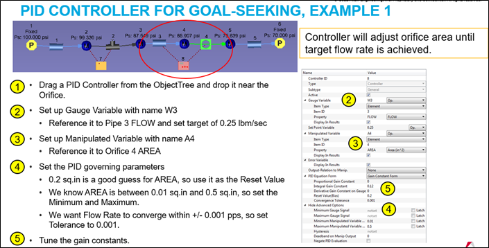
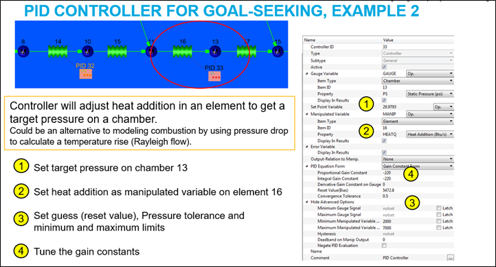
Select Gauge Variable. The model result that is the target of the PID controller.
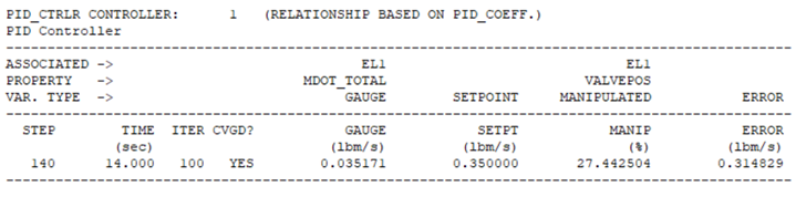
Define the Set Point (target) value. The target value for the gauge variable. It must be in English units. For the figure above, the target mass flow for element 1 is 0.35 lbm/sec.
Select the Manipulated Variable. The model input that is changed. The gauge variable must depend on the manipulated variable so that the PID controller works.
Set (also called tuning) the Gain Constants.
Set a Reset Value. The value of the manipulated variable that is close to the final result. For the figure above, a 5% valve position is close to the input that produces the Set Point result. If the input has a unit, then the Reset Value must be in English units. Also, it helps (not a requirement) to set the input value to the Reset Value. The valve position for element 1 is set to 5% in the Property Editor.
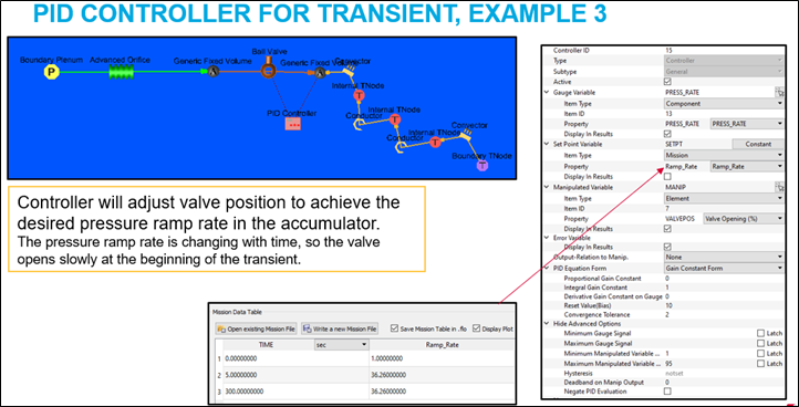
Set the Convergence Tolerance. The error, e(t), must decrease to this amount before convergence is declared. PID convergence works differently for a steady-state and a transient analysis. A steady-state analysis does not converge until the PID convergence tolerance is achieved. A transient analysis continues to the next time step, even if the PID convergence is not achieved. Adjust the transient run convergence behavior using the controls at the bottom of the PID controller window. The gain constants can be adjusted to get the PID closer to convergence during a transient analyss.
Variable Bounds (optional). The minimum and maximum manipulated variable bounds are useful. They can limit the PID to use physical values. For the figure above, the valve position is limited to between 1% and 100%. These must use English units if the variable has a unit. LATCH keeps the value at the bound value for the entire run if the limit is exceeded. Do not use LATCH if you want the controller to change a value, even if the limit is reached.
Deadband on Manip (optional). Only change the manipulated variable if the delta exceeds the deadband limit.
Negate PID Evaluation (optional). Select if the gauge variable has an inverse relationship with the manipulated variable. For example, if the gauge flow rate is reduced when the valve position was increased, check this value.

Tune the PID Controller Gain Constants

Tuning the PID controller gain constants can be difficult. The gain constants are model-dependent and take some experimentation to find a good set of values. Follow these tips:

Start with the proportional, K_p, and derivative, K_d, constants = 0 and use a nonzero integral, K_i, constant.
Start with a low K_i (like .01) and see if the sign is correct. If the model diverges, click Negate PID Evaluation.
The low K_i from hint 2 may not be large enough for the model to converge. Try larger values until convergence is acceptable. If the gain constants are too big, the controller may change the manipulated input too much and pass the target. The larger the gain constant, the faster the target is reached, but there is also an increased chance of passing the target (convergence problems).
Nonzero K_p and K_d may be needed if the model does not respond well to only the nonzero K_i. A nonzero K_p should be tried before also trying a nonzero K_d.
See the convhist_fi.out file for information on the controller convergence throughout the analysis. The model Debug Level provides useful information.

Figure 2.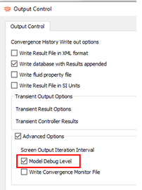

Additional line in convhist_fi.out:
Figure 3.

PID

The controller component number.

SPT

The set point (target) value.

GGE

The gauge variable value.

ER

The error value (SPT-GGE).

MAN

The manipulated value.

Controller Input


Index	UI Name (.flo label)	Description
1	Type (CPTYPE)	Component Type. 5=Controller
2	(SUBTYPE)	The type of controller: “FEEDFWD”, “MSSN_BC”, “PID”
3	Active (ACTIVE)	Active or Inactive option for the controller
4	Debug (DEBUG)	ON: Display detailed controller calculation results in the .res file. OFF: Only the output of the controller properties are displayed.
5	Relation Type 1 (RELATION1)	“TABLE1D”, “TABLE2D”, “CONSTANT”, “LINEAR”, “POLYNOM”, “PIDCOEF”, “PYFUNCT”
6	Relation Type 2 (RELATION2)	Currently not applicable; planned for future release.
7	Name (VARNAME)	Gauge and Manipulated names, which you can change.
8	(VARTYPE)	Controller input types: “GAUGE”, “MANIP”, “MISSION”, “SETPT”, “ERROR”
9	(ACT)	Active or Inactive option for the Manipulated or Gauge Variable
10	Relaxation Factor (DAMP/VAL)	Damping factor used to smooth out the calculation; value between 0.01 and 1.0. For “SETPT”, this is the value of the target.
11	Entity (ITEMTYPE)	Flow or thermal component that is defined as a gauge or manipulated variable in the controller to be considered or affected during the run time. “ELEMENT”, “CHAMBER”, “MISSION”, “COMPONENT”, “THERMAL”
12	ID	Chamber/Element/Component ID or Thermal Network ID
13	IDX1	List of Flow Component specific properties. For example, station number for some Tube element properties. Thermal Component type – Tnode, Conductor, Convector, Radiator, Heat Flow
14	IDX2	List of Flow Component specific properties. For example, circumferential wall side ID for some Incompressible Tube properties. Thermal Component ID
15	IDX3	List of specific properties. For example, left or right emissivity value of a two surface radiator.
16	Property (PROPERTY)	Property of the selected entity that is counted (as GAUGE) or altered (as MANIP) during the simulation. See the full list of available items in this file: <installation_directory>\Resources\misc_solver_files\controller_working_get_set.dat
17	Unit (UNIT_SET)	Property unit to be used for the variable in a Python script or tables.
18	Transient Convergence Check (CHECK_CONVERGENCE)	TRUE = Solver continues to iterate on solution until PID convergence criteria are met (default). FALSE = Solver declares time step converged, even if PID convergence criteria are not met.
19	Ignore convergence after % max iter (FRAC_ITER_FOR_CONVERGENCE)	If CHECK_CONVERGENCE=TRUE, the solver checks FRAC_ITER_FOR_CONVERGENCE to see if the solver can declare convergence, even if the PID controller is not converged. If the current iteration is greater than the maximum number of iterations * FRAC_ITER_FOR_CONVERGENCE/100, then the solver can converge without PID convergence. Default = 10%.

Controller Output

The figures below demonstrate the simulation examples that include controllers with various types, relation options, flow and/or thermal components, and properties.

Figure 4. PID controller that adjusts valve position to achieve the desired flowrate.

Examples