Inputs
1. Introduction
The total number of user inputs is equal to 16.
Among these inputs, 7 are standard inputs and 9 are advanced inputs.
2. Standard inputs
2.1 Line-Line voltage, rms
The rms value of the Line-Line voltage supplying the machine: “ Line-Line voltage, rms” ( Line-Line voltage, rms value ) must be provided.
When you run the test Characterization / Model /Basic twice consecutively by only changing the line-line voltage, the results you get at the end of the second run are wrong.
- If you run the test only once,
- or if you modify the voltage and the frequency at the same time,
- or if you modify other user input parameters but not the voltage,
In these three conditions the results will be right.
So that, the workaround consists in performing the second computation with not only a new value of the voltage but also a new value of the frequency very close to the one initially considered.
For instance, 50.001 Hz instead of 50.0 Hz.
In that case our internal process will consider that the line-line voltage has also been modified.
2.2 Power supply frequency
The value of the power supply frequency of the machine: “ Power supply frequency ” ( Power supply frequency ) must be provided.
The power supply frequency is the electrical frequency applied at the terminals of the machine.
2.3 Model refinement
A refinement of the initial model can be performed. The user’s input “ Model refinement ” ( Refinement to improve the original model ) gives three possibilities to the user:
-
Model refinement = None
No refinement will be performed.
-
Model refinement = Fitting
This choice gives to the user the capability to refine parameters of the equivalent scheme automatically for improving the results.
Note: The criteria for adjusting the parameters is to minimize the difference between results got with the model and those got with Finite Element computation. The three reference quantities for comparing results are the mechanical torque, the stator current and the reactive power. -
Model refinement = X-Factor
When “X-Factor” is selected, a list of X-Factors to be applied to each parameter of the equivalent scheme must be defined by using the next field: “X-Factors to be applied” and by clicking on the button “Set values”.
The second one, “ X-Factor ” ( X-Factor ) gives to the user the capability to adjust the parameter of the equivalent scheme manually. The manual adjustment is made thanks to X-Factor parameters which must be filled in the field “ X-Factor ”.
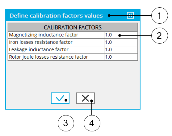 |
|
| Model refinement = X-Factor | |
| 1 | Select the “X-Factor” option. |
| 2 | Click the button “Set values” in the field “X-Factors to be applied” to open a dialog box to define the X-Factors to be applied on each parameter of the equivalent scheme. |
| 3 | Button to validate and consider the user inputs |
| 4 | Button to run the computation |
2.4 X-Factors
When “ Model refinement ” ( Refinements to improve the original model ) is set to “ X-Factor ” ( X-Factor ), “ X-Factors ” must be provided ( X-Factors applied on electrical components ). When the user clicks on “ Set values ” a dialog box appears allowing the user to set X-Factors values.
There are four X-Factors, “Magnetizing inductance factor”, “Iron loss resistance factor”, “Leakage inductance factor” and “Rotor Joule loss resistance factor”.
2.5 Model evaluation
An evaluation of the original model can be performed. The user’s input “ Model evaluation ” ( Model evaluation for a new set of voltage and frequency ) gives two possibilities to the user:
Model evaluation = Yes
The evaluation of the model accuracy is performed with the current model which has been characterized in the previous steps. Based on the model, quantities like mechanical torque, stator current, power factor… are computed and displayed.-
Model evaluation = Yes /w FE
When “ Yes W/ FE ” (Yes with finite element comparison) is selected, the evaluation of the model accuracy is performed with the current model which has been characterized in the previous steps.
However, quantities like mechanical torque, stator current, power factor… are computed, displayed and compared to results obtained with the Finite Element computations.
2.6 Operating Line-Line voltage
The rms value of the operating Line-Line voltage “ Op. Line-Line voltage, rms ” ( Operating Line-Line voltage to evaluate the equivalent scheme, rms value) must be provided.
This value allows to perform additional analysis at the targeted voltage.
2.7 Operating power supply frequency
The value of the operating power supply frequency “ Op. power supply freq. ” ( Operating power supply frequency to evaluate the equivalent scheme ) must be provided.
This value allows to perform additional analysis at the targeted frequency.
3. Advanced inputs
3.1 Model computation mode
There are 2 ways to identify the linear model of the induction machine.
An automatic process can be applied to determine automatically the two needed parameters to perform the test: “Locked rotor line current” and “Locked rotor slip”
In this case, the model computation mode should be “ Auto. ” ( Automatic )
A user process where the user must provide his own values for the two parameters “Locked rotor line current” and “Locked rotor slip”.
In this case, the model computation mode should be “ User ” ( User ).
3.2 Locked rotor line current, rms
When the choice of model computation mode is “User”, the rms value of the line current supplying the machine during the locked rotor test “ Lock rotor line current, rms ” ( Locked rotor line current, rms value required for the lock rotor computation ) must be provided. This value allows to identify the model at a targeted point.
3.3 Locked rotor slip for computing the reduced power supply frequency
If the advance parameter “ Model computation mode ” is set to “ User ”, the value of slip needed to compute the reduce power supply frequency during the locked rotor test “ Lock rotor slip ” ( Slip value needed to compute the reduced power supply frequency required for the lock rotor computation ) must be provided. This value allows to identify the model at a targeted point.
3.4 Slip distribution mode
The computation of the test is performed by considering a distribution of computed points. The user’s input “ Slip distribution mode ” ( Select the method for the distribution of computed points ) gives three possibilities to the user:
-
Slip distribution mode = Logarithmic
When “Logarithmic” is selected, the distribution of the computed points is automatically done. The number of computations to be done in the slip range must be set in the next field: “No. comp. in slip range”.
-
Slip distribution mode = Linear
When “Linear” is selected, the distribution of the computed points is automatically done. The number of computations to be done in the slip range must be set in the next field: “No. comp. in slip range”.
-
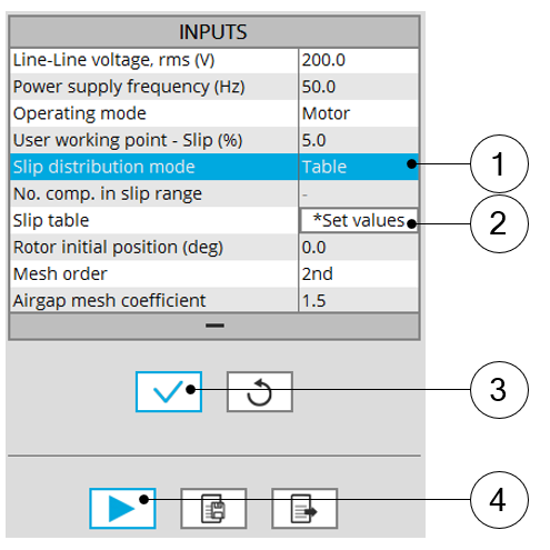
Slip distribution mode = Table
When “Table” is selected, the list of slips to be considered must be defined by using the next field: “Slip table” and by clicking on the button “Set values”.
Two ways are possible to fill the table: either filling the table line by line or by importing an excel file where all the slips to be considered are defined.
 |
|
| Slip distribution mode = Table | |
| 1 | Select the “Table” option. |
| 2 | Click the button “Set values” in the field “Slip table” to open a dialog box to define the list of slips to be considered.Refer to the next illustration which shows how to fill the Slip table. |
| 3 | Button to validate and consider the user inputs |
| 4 | Button to run the computation |
 |
|
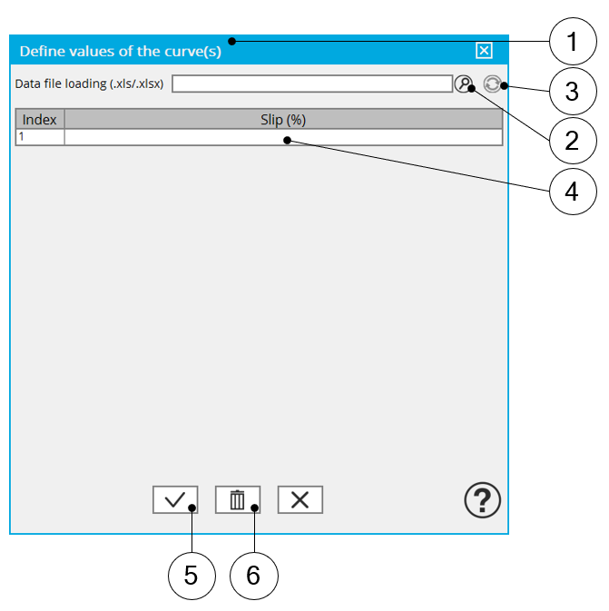
| Slip distribution mode = Table – Dialog box to define the list of slips | |
| 1 | Dialog box opened after clicked on the button “Set values” in the field “Slip table” |
| 2 | Browse the folder to select an Excel file which is defined the list of slips |
| 3 | Button to refresh the table data when the considered Excel file has been modified |
| 4 | Fields to be filled with data to describe the slips to be considered |
| 5 | Button to apply the inputs |
| 6 | Button to erase the data table |
Excel template used to import a list of slips is stored in the folder Resource/Template in the installation folder of FluxMotor. An example of this template is displayed below.
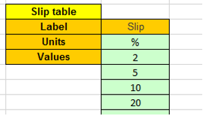 |
| Excel file template to define the list of slips |
3.5 Number of Finite Element computations
To compute the T(Slip) curve using Finite Element, the user input “ No. FE computations ” ( Number of Finite Element computations ) must be provided.
This input is required in the internal processes when the following modes are used:
- “Model computation mode” - “”
- “Refinement for original model” - “Fitting”
- “Model evaluation” – “Yes W. FE”
“ No. FE computations ” influences the accuracy of results and the computation time.
The default value is equal to 15. This value provides a good compromise between the accuracy of results and computation time.
3.6 Slip table
When the choice of point distribution mode is “ Table ”, the list of slips to be considered must be provided. Refer to the above section 3) Slip distribution mode = Table.
3.7 Skew model – Number of layers
When the rotor bars or the stator slots are skewed, the number of layers used in Flux Skew environment to model the machine can be modified: “ Skew model - No. of layers” ( Number of layers for modelling the skewing in Flux Skew environment ).
3.8 Rotor initial position
The initial position of the rotor considered for computation can be set by the user in the field « Rotor initial position » ( Rotor initial position ). The default value is equal to 0.
The range of possible values is [-360, 360].
The rotor initial position has an impact only on the induction curve in the air gap.
3.9 Mesh order
To get the results, the original computation is performed by using a Finite Element Modeling. The geometry of the machine is automatically meshed.
Two levels of meshing can be considered for this finite element calculation: first order and second order.
This parameter influences the accuracy of results and the computation time.
By default, second order mesh is used.
3.10 Airgap mesh coefficient
The advanced user input “ Airgap mesh coefficient ” is a coefficient which adjusts the size of mesh elements inside the airgap. When the value of “ Airgap mesh coefficient ” decreases, the mesh elements get smaller, leading to a higher mesh density inside the airgap, increasing the computation accuracy.
The imposed Mesh Point (size of mesh elements touching points of the geometry) is described with the following parameters:
MeshPoint = (airgap) x (airgap mesh coefficient)
Airgap mesh coefficient is set to 1.5 by default.
The variation range of values for this parameter is [0.05; 2].
0.05 giving a very high mesh density and 2 giving a very coarse mesh density.
However, this always leads to a huge number of nodes in the corresponding finite element model. So, it means a need of huge numerical memory and increases the computation time considerably.