Inputs
1. Introduction
The total number of user inputs is equal to 14.
Among these inputs, 8 are standard inputs and 6 are advanced inputs.
2. Standard inputs
Current definition mode
There are two common ways to define the electrical current.
Electrical current can be defined by the current density in electric conductors.
In this case, the current definition mode should be « Density »
Electric current can be defined directly by indicating the value of the maximum line current (the rms value is required).
In this case, the current definition mode should be « Current »
Maximum line current, rms
When the choice of the current definition mode is “ Current ”, the maximum rms value of the line current supplied to the machine: “ Max. line current, rms” ( Maximum line current, rms value ) must be provided.
Maximum current density, rms
When the choice of current definition mode is “ Density ”, the rms value of the maximum current density in electric conductors “ Max. current dens., rms” ( Maximum current density in conductors, rms value ) must be provided.
Maximum Line-Line voltage, rms
The rms value of the maximum line-line voltage supplying to the machine: “ Max. Line-Line voltage, rms” ( Maximum Line-Line voltage, rms value ) must be provided.
Command modes – Introduction
Whatever is the applied command mode, the first step of the process consists of computing the torque-speed curve and the second step is to compute the efficiency map bounded by the torque-speed curve.
In function of the command mode, the applied process of computation is different to obtain curves and maps.
For additional information on this topic see the section dedicated to the command modes
Maximum speed
The computation and analysis of the torque-speed curves are performed over a given speed range.
The maximum allowed value for the « Maximum speed » corresponds to 53000 rad/s - about 506000 rpm.
-
Case 1 : The maximum speed is lower than the base speed N base (corner point speed of the torque-speed curve) N max < N base .
In that case, whatever is the command mode (MTPA or MTPV), the behavior of the machine will be studied over the speed range [0, N max ].
That allows the user to precisely choose the range of speed to be considered for computing and displaying the torque-speed curve and especially maps like efficiency map.
- Case 2 : The maximum speed is greater than the base speed
(corner point speed) N max > N base
The relevance of the maximum speed given by the user is analyzed to evaluate if it is reachable by the machine.
If the user maximum speed is unreachable by the machine, the correction of this value is automatically performed.
The resulting new maximum speed is linked to a limit torque. This limit torque is obtained by applying a reduction coefficient to the base point torque.
Rotor position dependency
Additional losses
“Additional losses” input is not available in the current version (The input label is written in grey).
User working point(s) analysis
It is possible to perform additional analysis on working point(s) located under the torque-speed curve. The user’s input “ User working point(s) analysis ” (additional analysis on working point(s)) gives three possibilities to the user:
-
User working point(s) analysis = None (=default mode)
This corresponds to the basic configuration of the test, with no additional working point analysis.
-
User working point(s) analysis = Single point
This allows computing the machine performance on a working point which must be specified by the user with the targeted speed and torque. In that case the next two fields must be filled with the targeted speed and mechanical torque.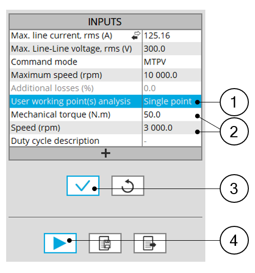
User working point analysis = Single point 1 Select the “Single point” option to perform a computation on one working point. 2 Define the targeted working point mechanical torque and speed. 3 Button to validate and consider the user inputs 4 Button to run the computation -
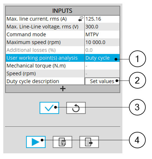
User working point(s) analysis = Duty cycle
This allows computing the machine performance all over a considered duty cycle.
This duty cycle must be defined by using the next field: "Duty cycle description" and by clicking on the button "Set values".
Two ways are possible to fill in the table: either filling in the table line by line or by importing an excel file which all the working points of the duty cycle are defined.
 |
|
| User working point analysis = Duty cycle | |
| 1 | Select the “Duty cycle” option |
| 2 | Click in the button “Set values” of the field “Duty cycle” to open a dialog box to define the duty cycle.Refer to the next illustration which shows how to fill the Duty cycle table. |
| 3 | Button to validate the user input data |
| 4 | Button to run the computations |
 |
|
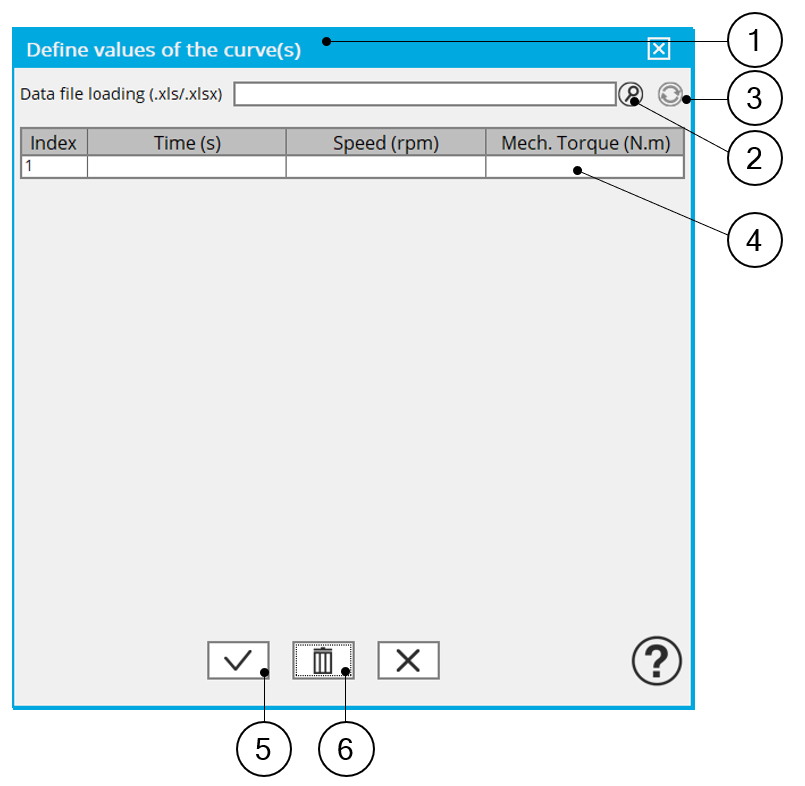
| User working point analysis = Duty cycle – Dialog box to define the duty cycle | |
| 1 | Dialog box opened after having clicked on the button “Set values” in the field “Cycle description” |
| 2 | Browse the folder to select an Excel file which is described the duty cycle |
| 3 | Button to refresh the table data when the considered Excel file has been modified |
| 4 | Fields to be filled with data to describe the duty cycle to be considered |
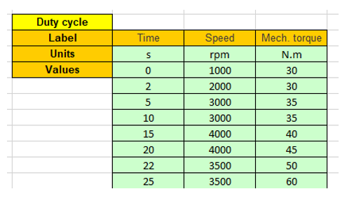 |
| Excel file template to define the duty cycle |
User working point(s) analysis with thermal solving
When thermal solving has been selected in the settings, it is mandatory to define the driving cycle with a list of working points.
This duty cycle must be defined by using the field: "Duty cycle description" and by clicking on the button "Set values".
Two ways are possible to fill in the table: either filling in the table line by line or by importing an Excel file which all the working points of the duty cycle are defined. The Excel sheet format will be the same than in the previous section.
 |
|
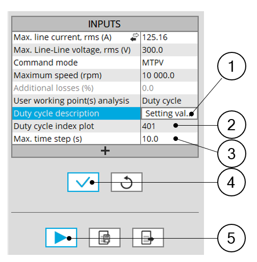
| User working point analysis = Duty cycle | |
| 1 | The “Duty cycle” option is mandatory when thermal solving is selectedClick in the button “Set values” of the field “Duty cycle” to open a dialog box to define the duty cycle.Refer to the next illustration which shows how to fill the Duty cycle table. |
| 2 | The index plot allows us to select a working point of the cycle for displaying data and maps which are corresponding to its thermal properties. |
| 3 | Maximum time step which is considered to discretize the driving cycle sequences. There will be no time step greater than the value written in that field (10 s in our example).The minimum value = 0.01s, the maximum value = 3600s.The default value = 10s |
| 4 | Button to validate the user input data |
| 5 | Button to run the computations |
3. Advanced inputs
Number of computed electrical periods
The user input “No. computed elec. periods” (Number of computed electrical periods only required with rotor position dependency set to “Yes”) influences the computation time of the results.
Number of computations for J d , J q
First, it is needed to compute the D-axis and Q-axis flux linkage in the J d - J q plane.
To get maps in the J d - J q plane, a grid is defined. The number of computation points along the d-axis and q-axis can be defined with the user input « No. Comp. for J d , J q » (Number of computations for D-axis and Q-axis currents) .
The default value is equal to 5. This default value provides a good compromise between accuracy and computation time. The minimum allowed value is 5.
Number of computations for speed
The “ No. comp. for speed” ( Number of computations for speed ) corresponds to the number of points to be considered in the speed range from 0 to the maximum speed.
Half of these points are distributed from 0 to the base speed. The remaining points are distributed from the base speed to the maximum speed.
In both cases, base speed is considered as an additional point.
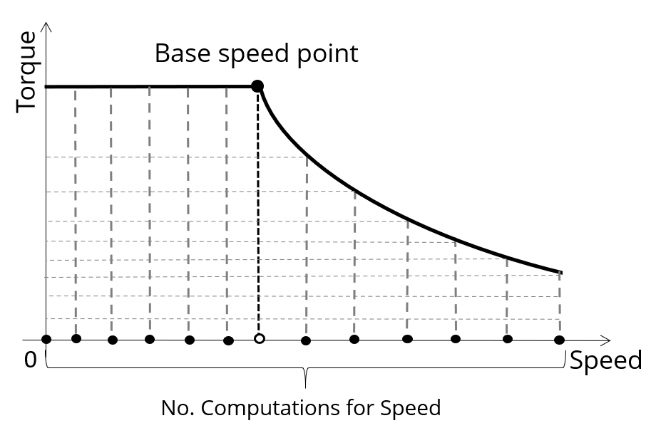 |
| Definition of the number of computations for speed |
The default value is equal to 15, the minimum allowed value is 5. The maximum recommended value is 40.
Number of computations for torque
For the speed range [N base ; N max. ], the number of computations for torque is imposed by the number of computations for speed in the speed range [N base ; N max. ] (Red points in the image shown below).
The advanced user input parameter “ No. comp. for torque ” allows to finalize the grid within the torque range [0, T (N max. )] at the maximum speed (Black points in the image shown below).
The default value is equal to 7. The minimum allowed value is 3. The maximum recommended value is 20.
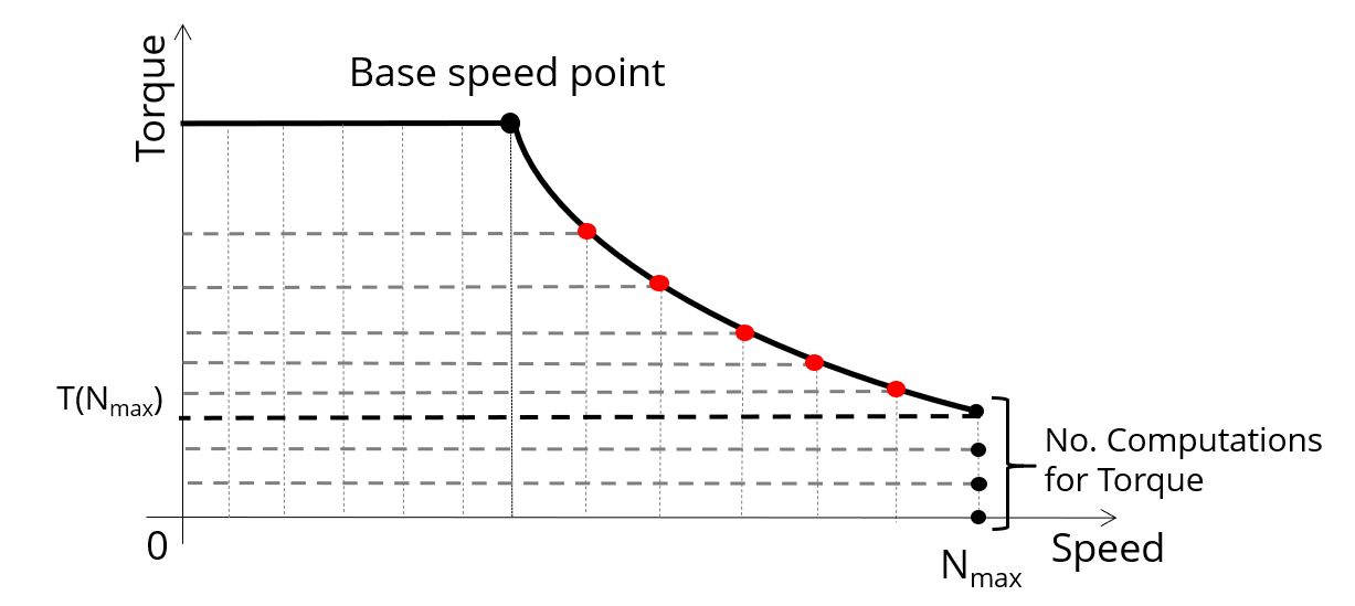 |
| Definition of the number of computations for torque – MTPV command mode |
Rotor initial position
By default, the “ Rotor initial position ” is set to “ Auto ”.
When the “ Rotor initial position mode ” is set to “ Auto ”, the initial position of the rotor is automatically defined by an internal computation process.
The resulting relative angular position corresponds to the alignment between the axis of the stator phase 1 (reference phase) and the direct axis of the rotor north pole.
When the “ Rotor initial position ” is set to “User input” (i.e. toggle button on the right), the initial position of the rotor considered for computation must be set by the user in the field « Rotor initial position ». The default value is equal to 0. The range of possible values is [-360, 360].
For more details, please refer to the document: dedicated to the "Rotor and stator relative position”.
Skew model – Number of layers
When the rotor magnets or the stator slots are skewed, the number of layers used in Flux Skew environment to model the machine can be modified: “ Skew model - No. of layers” ( Number of layers for modelling the skewing in Flux Skew environment ).
Mesh order
To get the results, the original computation is performed using a Finite Element Modeling.
Two levels of meshing can be considered for this finite element calculation: first order and second order.
This parameter influences the accuracy of results and the computation time.
By default, second order mesh is used.
Airgap mesh coefficient
The advanced user input “ Airgap mesh coefficient ” is a coefficient which adjusts the size of mesh elements inside the airgap. When the value of “ Airgap mesh coefficient ” decreases, the mesh elements get smaller, leading to a higher mesh density inside the airgap and increasing the computation accuracy.
The imposed Mesh Point (size of mesh elements touching points of the geometry), inside the Flux ® , is described as:
MeshPoint = (airgap) x (airgap mesh coefficient)
Airgap mesh coefficient is set to 1.5 by default.
The variation range of values for this parameter is [0.05; 2].
0.05 giving a very high mesh density and 2 giving a very coarse mesh density.
However, this always leads to a huge number of nodes in the corresponding finite element model. So, it means a need of huge numerical memory and increases the computation time considerably.