Inputs

1. Introduction

The total number of inputs is equal to 7.

Among these inputs, 1 is a standard input and 6 are advanced inputs.

Note that the standard input corresponds to a table to be filled with a set of working point described as indicated in the following section.

2. Standard inputs

2.1 U-f-N description

The “ U-f-N description ” allows to define several working points.

The description must be defined by clicking on the button “Set values”.

Then, two ways are possible to fill in the table: either filling the table line per line or by importing an Excel file in which all the working points to be considered are defined.

Each working point is described by the following data:

1. Line current, rms

   The rms value of the line current supplying the machine: “ Line current, rms” ( Line current, rms value ) must be provided.

   Note: The number of parallel paths and the winding connections are automatically considered in the results.

2. Power supply frequency

   The value of the power supply frequency of the machine: “ Power supply frequency ” ( Power supply frequency ) must be provided.

   The power supply frequency is the electrical frequency applied at the terminals of the machine.

2.2 Definition mode

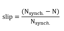
There are 2 common ways to define the working point. It can be defined by indicating the slip “ Slip ” or by defining the operating speed of the machine “ Speed ”.

2.3 Slip

When the choice of definition mode is “Slip” , the value of machine’s slip “Slip” ( Slip ) must be provided.

Unit can be % or PU.

2.4 Speed

When the choice of definition mode is “Speed” , the value of operating speed “Speed” ( Speed ) must be provided.

2.5 Process to define the list of working points

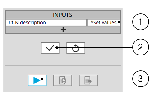
List of working points to be defined
1	Click on the button “Set values” of the field “ U, f, N description” to define the working points in a dialog box. Refer to the next illustration which shows how to fill the working point table.
2	Button to validate the user input data
3	Button to run the computations

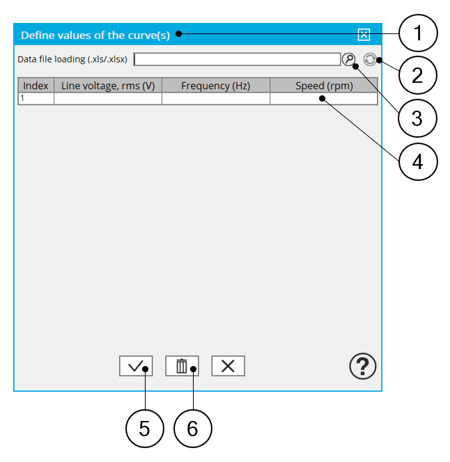
Dialog box to define the list of working points
1	Dialog box opened after having clicked on the button “Set values” in the field “Cycle description”
2	Browse the folder to select an Excel file to define the working points to be considered
3	Button to refresh the table data when the considered Excel file has been modified
4	Fields to be filled with data to describe the list of working points to be considered

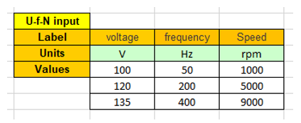Excel file template to define the list of working points

3. Advanced input

3.1 Maximum engine order / No. Points per electrical period

Two kinds of inputs are possible:

Define the Max. engine order ( Maximum engine order ) or the No. points / elec. Period ( Number of points per electric period ).

When decomposing the Maxwell pressure, applied on the stator, to get its harmonic contributions, the “ max. engine order ” ( Maximum engine order ) is required to compute its decomposition in function of the time.

At a practical point of view, when the maximum engine order is equal to N, that leads to consider 2*N computation points over a complete rotation period of the rotor.

3.2 Maximum mode / spatial order

The “ max. mode / spatial order ” ( Maximum mode / spatial order ) input allows the user to define the number of modes to be considered for the acoustic structural analysis. If the user selects 25, it means that the highest number of lobes in the stator deformation will be equal to 25 lobes. All deformations corresponding to more than 25 lobes will be dismissed.

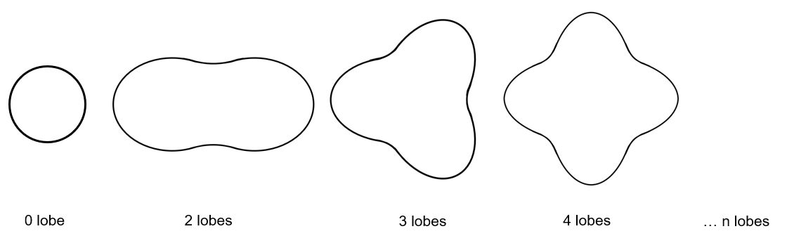Number of lobes of the stator mechanical structure

3.3 Number of computations per tooth pitch

The “ No. comp./tooth pitch ” ( Number of computations per tooth pitch ) allows to choose the number of Maxwell pressure evaluations per tooth. The more points selected, the more accurate the Maxwell pressure harmonic decomposition will be.

3.4 Number of points for speed interpolation

The “ No. points for speed interpolation ” (Number of points for speed interpolation) allows to manage the computation of the sound power level per engine order. It allows to manage the data interpolation between the speeds indicated as inputs. Thanks to that, the curves “Sound power level per engine order versus speed” and “weighted sound power level versus speed” can have a better discretization which leads to a better displaying of the local peaks.

The default value is equal to 100. The range of possible values is [50,300]

3.5 Number of rotor turns

This input allows us to define the number of rotor revolutions to consider the slip as far as possible.

Higher is the number of rotor revolutions better will be the results. However, this value has a huge impact on the computation time.

The default value is equal to 5. This is a good compromise between computation time and quality of results.

The variation range of values for this parameter is [1; 10].

3.6 Mesh order

To get the results, the original computation is performed using a Finite Element Modeling .

Two levels of meshing can be considered for this finite element calculation: first order and second order.

This parameter influences the accuracy of results and the computation time.

By default, second order mesh is used.

3.7 Airgap mesh coefficient

The advanced user input “ Airgap mesh coefficient ” is a coefficient which adjusts the size of mesh elements inside the airgap. When the value of “ Airgap mesh coefficient ” decreases, the mesh elements get smaller, leading to a higher mesh density inside the airgap, increasing the computation accuracy.

The imposed Mesh Point (size of mesh elements touching points of the geometry) is described with the following parameters:

MeshPoint = (airgap) x (airgap mesh coefficient)

Airgap mesh coefficient is set to 1.5 by default.

The variation range of values for this parameter is [0.05; 2].

0.05 giving a very high mesh density and 2 giving a very coarse mesh density.