Basics of Ray-Optical Models

Primary Criterion for Ray-Optical Models

The mobile radio channel in urban environments is characterized by strong multipath propagation. Dominant propagation mechanisms in these scenarios are reflection, diffraction, shadowing by discrete obstacles and wave guiding effects in street canyons. With a ray-optical approach, it is possible to consider these effects in a propagation model.

As smaller wavelengths (higher frequencies) are considered, the wave propagation becomes similar to the propagation of light. A radio ray is assumed to propagate along a straight line influenced only by refraction, reflection, diffraction or scattering. These are the concepts of geometrical optics (GO). The criterion taken into account for this modeling approach is that the wavelength should be much smaller in comparison to the extents of the considered obstacles (buildings for urban environments). At the frequencies used for mobile communication networks, this criterion is sufficiently satisfied.

Specular Reflection

Specular reflection phenomena are the mechanism by which a ray is reflected at an angle equal to the incident angle. The reflected wave fields are related to the incident wave fields through a reflection coefficient which can be expressed as a matrix when the full polarimetric description of the wave field is taken into account. The most common expression for the reflection is the Fresnel reflection coefficient which is valid for an infinite boundary between two mediums, for example, between air and concrete. The Fresnel reflection coefficient depends on the incident wave field and upon the permittivity and conductivity of each medium. The application of the Fresnel reflection coefficient formulas is popular, and these equations are also applied in ProMan.

Figure 1. Specular reflection is where the incident angle is equal to the reflected angle.

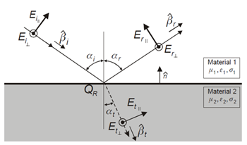
To calibrate the prediction model with measurements some ray-optical software tools consider an empirical reflection coefficient is varying with the incidence angle to simplify the calculations. Such an empirical approach is also available in ProMan.

The reflection loss in the empirical model depends on the angle of incidence (with respect to the perpendicular line of the wall) and the reflection loss defined in the material properties. For the reflection loss there is a linear decrease from full reflection loss at perpendicular incidence to half of the loss for grazing incidence. This means the defined reflection loss is used for perpendicular incidence and half of the loss for grazing incidence.

Figure 2. The reflection loss depends on the angle of incidence with respect to the perpendicular line of wall.

Diffraction

The diffraction process in ray theory is the propagation phenomena which explain the transition from the illuminated region to the shadow regions behind a corner or over rooftops. Diffraction by a single wedge can be solved in various ways: empirical formulas, perfectly absorbing wedge, geometrical theory of diffraction (GTD) or uniform theory of diffraction (UTD). The advantages and disadvantages of using either formulation are difficult to address since it may not be independent of the environments under investigation. However reasonable results are possible with either formulation. The various expressions differ mainly in the approximations being made on the surface boundaries of the wedge under consideration. One major difficulty is to express and use the proper boundaries in the derivation of the diffraction formulas. Another problem is the existence of wedges in real environments - the complexity of a real building corner or the building’s roof illustrates the modeling difficulties.

Despite these difficulties, however, diffraction around a corner or over rooftops are commonly modeled using the heuristic UTD formulas since they are well behaved in the illuminated/shadow transition region, and account for the polarization as well as for the wedge material. Therefore these formulas are also used in ProMan to calculate the diffraction coefficient.

Multiple Diffraction

For the case of multiple diffractions, the complexity increases dramatically. In the case of propagation over rooftops, the result of Walfisch and Ikegami has been used to produce the COST-Walfisch-Ikegami model. One method frequently applied to multiple diffraction problems is the UTD. The main problem with straightforward applications of the UTD is in many cases one edge is in the transition zones of the previous edges. Strictly speaking, this forbids the application of ray techniques, but in the spirit of the UTD, the principle of local illumination of an edge should be valid. At least to some approximate degree, a solution can be obtained which is quite accurate in most cases of practical interest.

The key point in the theory is to include slope diffraction, which is usually neglected as a higher order term in an asymptotic expansion, but in the transition zone diffraction, the term is of the same order as the ordinary amplitude diffraction terms. ProMan utilizes the UTD including slope diffraction for over rooftop propagation for the calculation of multiple diffractions. Also, there is an empirical diffraction model available which can easily be calibrated with measurements.

Scattering

Rough surfaces and finite surfaces (thus surfaces with small dimensions regarding the wavelength) scatter the incident energy in all directions with a radiation diagram which depends on the roughness and size of the surface or volume. The dispersion of energy through scattering means a decrease of the energy reflected in the specular direction.

One can account for the scattering process by simply decreasing the reflection coefficient. You can do this by multiplying it by a factor smaller than one which depends exponentially on the standard deviation of the surface roughness according to the Rayleigh theory.

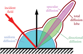
This roughness value represents the standard deviation of a Gaussian distribution, meaning that 68% of surface points are within plus or minus this value from the average surface height. The scattering intensity I_s at any observation point P above a rough surface S, is expressed in terms of the intensity of the incident field I_i, through the Bidirectional Reflectance Distribution Function (BRDF)¹².

The BRDF, denoted ρ and expressed in sr^-1, represents the spatial distribution of I_s (P) and is defined as the ratio of the scattering intensity in the direction (θ_s, θ_s) to the total incident intensity I_i in an elementary solid angle dω_i on the surface S in the direction θ_i (we note that ϕ_i = 0°). The BRDF is the sum of three components: specular ρ_sr, directional diffuse ρ_dd and uniform diffuse ρ_ud (see Figure 3).

Figure 3. The main BRDF components.

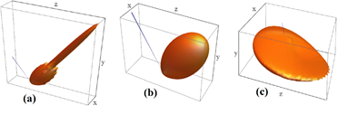
The surface roughness and the wavelength are used to compute the relative roughness $\frac{{\sigma }_0}{\lambda }$ , which tells us how rough a given surface is with respect to the wavelength of the incident field.

These profiles determine how narrow or large the resulting scattering lobe is, and the incident angle determines its directivity.

Figure 4. Scattering lobe for (a) low, (b) moderate, and (c) high surface roughness profiles.

Penetration and Absorption

Penetration loss due to building walls has been investigated and found very dependent on the particular system. Absorption due to trees or absorption by the human body is also propagation mechanisms difficult to quantify with precision. Therefore in the radio network planning process, adequate margins should be considered to ensure overall coverage.

Another absorption mechanism is the one due to atmospheric effects. These effects are usually neglected in propagation models for mobile communication applications at radio frequencies but are important when higher frequencies (for example, 60 GHz) are used.

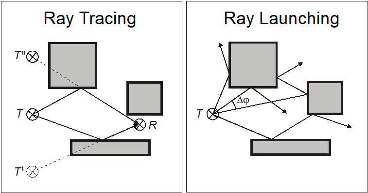
Ray Tracing Versus Ray Launching

Ray tracing computes all rays for each receiver point individually and guarantees the consideration of each wall as well as a constant resolution. The image principle is used to find all reflections. In the ray launching approach, the rays are launched from the transmitter with a constant angular increment. Thus ray launching might neglect a wall because it is very small and located between two rays. Different approaches to a better resolution with ray launching were proposed recently, but ray launching has still kept the disadvantage of a variable resolution depending on the distance to the transmitter. The only advantage of ray launching is the shorter computation time compared to standard ray-tracing algorithms (This is not valid for the intelligent ray tracing, which is much faster than ray launching). Figure 5 illustrates the differences between ray-tracing and ray launching.

Figure 5. Deterministic propagation models.

Regardless of the model that is used for the determination of the rays between the transmitter and the receiver, the received power has to be calculated by the superposition of all contributions. WinProp offers two options, uncorrelated (a statistical summation of contributions based on power considerations) and correlated (taking the phases into account). The latter is important in some multipath situations, but may often be undesired in urban scenarios because it will include the small-scale fading.