Profile Editor

View the Profile Editor (Time Dependent)

Click

on the motors or actuators microdialog to open the Profile Editor.

Tip:

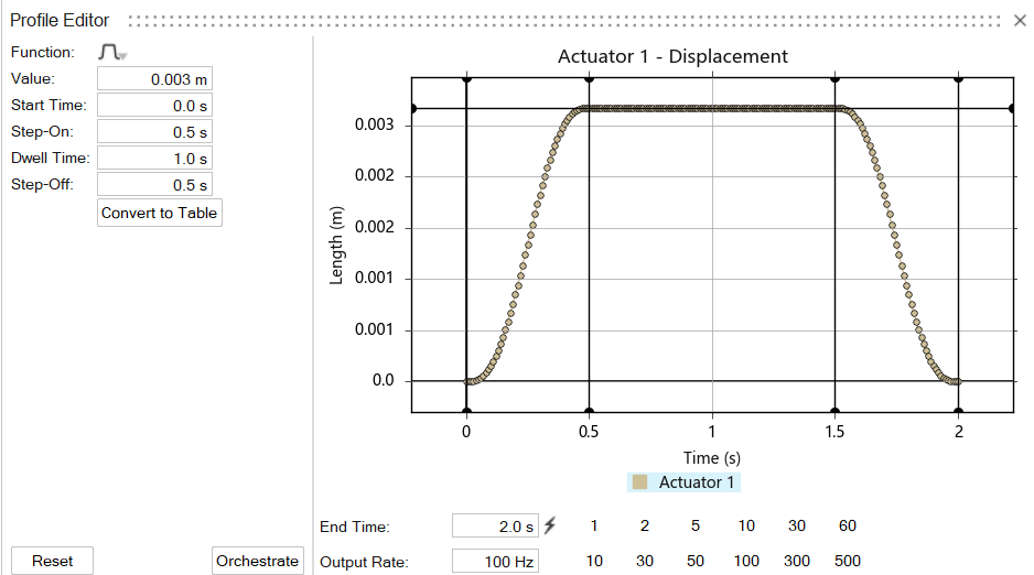
If you enter zero for the Value, the motor or actuator will be locked and the Profile Editor will become uneditable. To reverse this, double-click the motor or actuator in the modeling window to edit it, and click on the microdialog to unlock it
Click the Reset button to restore the current profile function to its default values
Certain profile functions have sliders under some parameters. You can click and drag a slider to shape the profile function.
Right-click on the plot and then click Export Image to export an image of the profile function.
Look closely at the Start Time setting when changing back and forth between profiles or when using the Convert to Table option.

Modify the Profile Function Interactively (Time Dependent)

Click and drag the plot sliders in the Profile Editor to reshape the profile function.

Sliders are highlighted as you hover over them with the mouse, and a memory curve shows the original shape.
The sliders can snap to grid lines or parameters on other profile functions. Press Alt to temporarily disable snapping.
Blue dashed lines, when visible, represent other profiles in use in the model. You can snap to features on those profiles as well.

Tip:

You can pan, zoom, and fit the plot. When zooming, use the Ctrl key to keep the x-axis fixed. Press F or double-click to fit the plot.
Clicking on the plot sliders also puts focus on the associated property. This makes it easy to gain more precise control by typing in a value.
For table functions, click and drag data points in the chart to modify them individually. You can also box select to move multiple data points simultaneously.
To provide better control when adjusting curves, the tool tip for time-based sliders shows the absolute time.
When your time unit is milliseconds, the Output Rate reports the value in kHz.

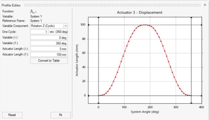
Specify the Variable Range or Cycle (State Dependent)

In the Profile Editor, specify the variable range or cycle over which the input function will be applied.

Option	Description
Function	Select a profile function. Supported functions include: Step Step Dwell Step Single Wave Oscillating Swept Sine Impulse Ramp Solver Expression Multi-Signal
Variable	The independent variable object (system, measure, motor, or actuator).
Reference Frame	The reference frame used by the variable component.
Variable Component	The independent variable component output that the state dependent object will monitor. Use the dropdown menu to access to the library of functions.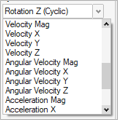
One Cycle (for cyclic rotations)	Specify the cycle range within which the V(i) and V(f) values fall. For example, a 4-stroke piston engine will experience combustion force every 2 revolutions (or 720 degrees) of the crankshaft.
Variable (i)	Enter the initial value of the independent variable object (system, measure, motor, or actuator).
Variable (f)	Enter the final value of the independent variable object (system, measure, motor, or actuator).
[Variable Object] Force (i)	Enter the initial value of the state dependent object.
[Variable Object] Force (f)	Enter the final value of the state dependent object.

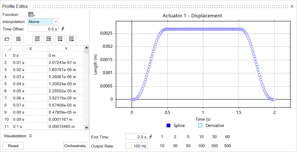
Convert a Profile Function to a Table

Convert a profile function to a table to modify data points and save them in a .csv file.

Select the Table function to convert a profile function to a table. Click Spline or Derivative in the legend to plot one or the other.

Option	Description
	Load values from a .csv file. Alternatively, you can drag and drop a valid .csv file onto the profile editor.
	Save data to a .csv file.
	Insert a value before the first data point.
	Insert a value after the selected data point.
	Insert a value after the last data point.
	Delete the selected data points.
Extrapolate	Linearly extrapolate the curve at both ends. The default is 10%.
Number of points	The number of interpolation points. The default is 1024 points. If the Spline curve does not appear to be passing through your data points, try increasing the Number of Points under the Visualization section.

Create Multi-Signal Profiles

The Multi-Signal function type in the Profile Editor allows you to quickly and easily define motor and actuator inputs comprising multiple time-based changes during a single motion analysis.

In the modeling window, click a motor or actuator.
In the microdialog, click the Profile Editor/Orchestrator icon .
The Profile Editor window opens.

Select Multi-Signal

from the Function dropdown list.

The Profile Editor window changes to Multi-Signal mode.

See the table below for signal editing options while in Multi-Signal mode: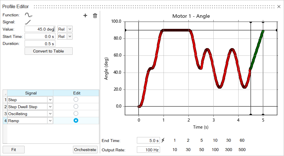

To	Do this	Notes
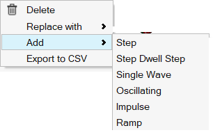
Add a signal function	Option 1: In the Profile Editor window, click the Add icon. The signal will be added after the currently selected curve. Option 2: Right-click a curve in the curve preview window. Choose Add from the context menu, then select a signal function type from the list. Value and Start Time can be defined as being Relative to the previous function’s Value or Start Time, or relative to absolute 0. 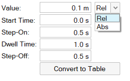Select the dropdown arrow next to Rel or Abs to change. Example: Function 1 is already defined with a Value of `60` rpm. A new function, which will reach a speed of `180` rpm, is defined after that. In this case, you have the option of defining the Value as either `120` Rel or `180` Abs.	Note: The simulation End Time shown under the curve preview window will automatically increase or decrease as functions are added or deleted.
Change a signal function type	Option 1: Select the dropdown arrow next to the signal you would like to change, then choose a new signal function type. Option 2: Right-click a curve in the curve preview window. Choose Replace with from the context menu, then select a new signal function type.
Delete a signal function	Option 1: Select the Edit button for the signal you would like to delete, then select Delete. Option 2: Right-click the curve of interest, then choose Delete from the context menu.
Edit a signal function	Option 1: Select the curve you would like to edit from the table or the curve preview window, then enter values directly into the corresponding fields. Option 2: Select the curve you would like to edit. In the curve preview window, left-click, hold and drag the horizontal or any of the vertical curve handles to dynamically change values.	Note: Dragging the handles for one function can affect the Start Time of the functions that follow. For example, if you wish to change the Start Time or Dwell Time of a function without affecting the Start Time of the functions that follow, hold the Ctrl key while dragging the function handle in the curve preview window.
Export a .csv file of a curve	Right-click a curve in the preview window, then choose Export to CSV.

Use the Profile Orchestrator

The Profile Orchestrator is an extension of the Profile Editor where you can view, edit, and organize model inputs in a single window.

Click Orchestrate.
The Profile Editor window switches to the Profile Orchestrator window.
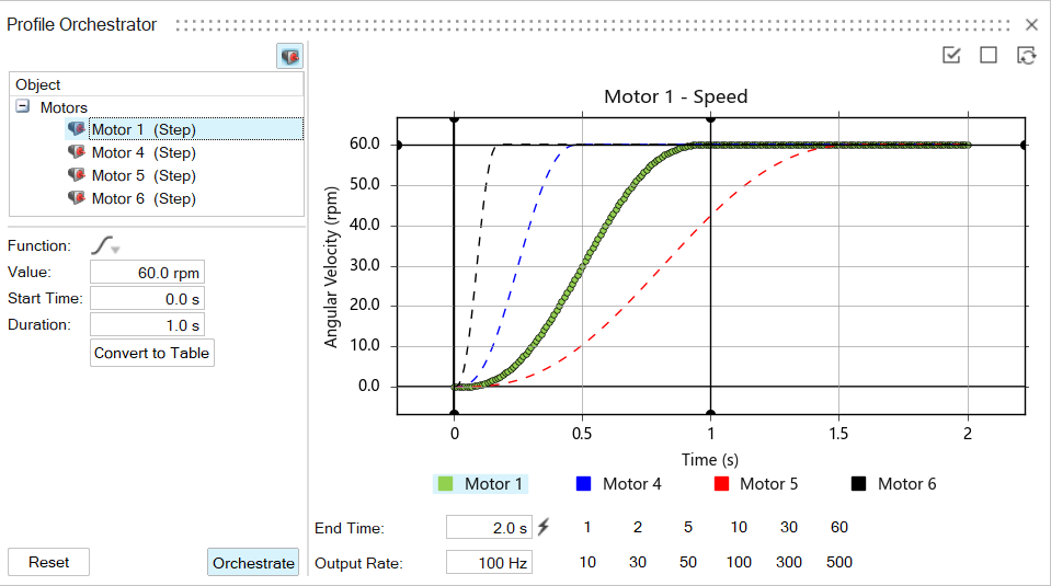
In the Object browser, select an input Object you would like to edit. You can also directly click a curve that you would like to edit in the plot to make it the active curve.
Note: The legend and name for the active curve will always appear in the leftmost position in the legend beneath the plot window.
Enter values in the Function editor, or drag the interactive handles surrounding the active curve on the plot to make adjustments.

To	Do this
Filter the plot display by input type	Click the Show/Hide Actuators or Show/Hide Motors icon to the right of the Object browser. Note: A motor or actuator must be present in the model when you run your analysis in order for the corresponding Show/Hide icon to appear in the Profile Orchestrator.
View all inputs	Click .
Hide all inputs	Click .
Reverse all inputs	Click .
Show/Hide individual curves	Click the colored labels on the legend underneath the plot.
Multi-select inputs	Ctrl+click multi-select is available only for inputs of the same Function type, and only for changing the values of the function. You cannot select inputs of different function types and change them all simultaneously to a different type. To change multiple input types simultaneously, multi-select the inputs in the Model Browser, and then use the Property Editor to change the Type.
Switch from the Profile Orchestrator to the Profile Editor	Click Orchestrate.

Tip:

Since the coordination of timing is the main focus of the Profile Orchestrator, curves of different input types (speed, angle, torque, etc.) are normalized to the active (selected) input, so they can be viewed on the same plot without needing multiple axis legends. This means the maximum Y value for the normalized curves will be in line with the maximum Y value of the active curve.
Table-based profiles are single curve view only in the Orchestrator. Currently, they cannot be viewed simultaneously with other input types.
If you hide a motor or actuator in your model, the input curve will still display in the Profile Orchestrator plot, but the corresponding icon in the Objects browser will be grayed out. Although the entity is hidden in the model, it is available for modification when synchronizing against other inputs.

Shortcuts

To	Do This
Disable snaps temporarily	Press Alt
Pan the plot	Click and drag the right mouse button.
Zoom in the plot	Use the scroll wheel on the mouse. Press Ctrl + scroll to keep the x-axis fixed (zoom y). Press Shift + scroll to keep the y-axis fixed (zoom x).
Fit the plot	Press F or double-click the plot.