OS-V: 0800 Hyperelastic Material Verification

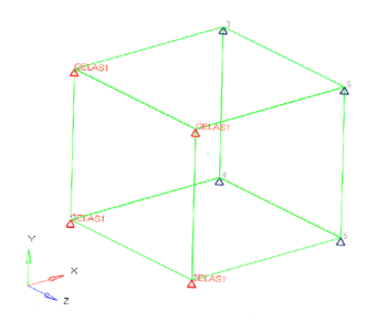
Examines the hyperelastic behavior of a hexahedral element under enforced displacement using different material models such as Arruda Boyce, reduced polynomial, Yeoh and Ogden model.

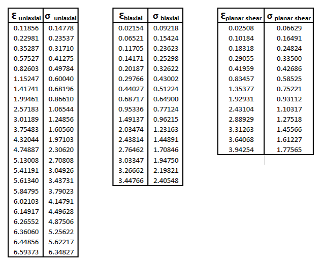
In 1944, L.G.R. Treloar 1 performed experiments on 8% rubber to obtain the uniaxial stress-strain curve which has been digitized and utilized for this simulation.

Model Files

Before you begin, copy the file(s) used in this problem to your working directory.

Benchmark Model

A single hexahedral element with 8-node CHEXA is used to perform the hyperelastic simulation. The element is of size 10 x 10 x 10 millimeters. The nodes 1, 2, 7, and 8 are constrained through zero-length CLEAS elements in 5 degrees of freedom (2,3,4,5,6) and a small value of spring stiffness is assigned to restrain the element (this does not affect the results of the simulation). Enforced displacement of 70 mm in DOF 1 is applied on nodes 3, 4, 5, and 6 using SPCD entry. The material stress-strain curve for 8% sulphur rubber has been digitized from the Treloar 1 paper.


Figure 1. 1-Element FE Model

Units: mm, s, Mg, N, MPa

Material

The MATHE Bulk Data Entry is used to input hyperelastic material data for the model.
Field
Model
Identifies material model
NU (Poisson's Ratio)
Both 0.4997 and 0.495 values can be used
0.4997 demonstrates a better fit for the incompressible rubber material
TAB1
Defines the Uniaxial tension-compression data
TAB2
Defines Equi-biaxial data
TAB4
Defines Shear data
Required engineering stress versus strain material data is generated from test data as curve input for different material laws. The hyperelastic data gathered by Treloar for 8% sulfur rubber test data is used. Figure 2 and Figure 3 show the Treloar test data for the 3 strain states most important in characterizing a hyperelastic material, uniaxial tension, equal biaxial extension and pure shear. 2


Figure 2. Treloar Test Data


Figure 3. Digitized Treloar Test Data 8% Sulphur Rubber: Uniaxial, Biaxial and Planar Shear

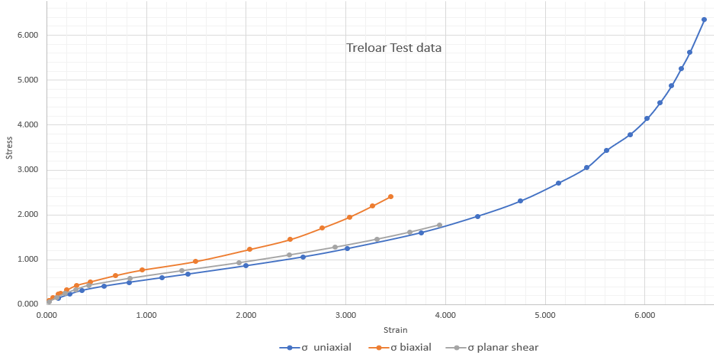
For RPOLY material model, 3 test data Uniaxial, Biaxial, and Planar Stress-Strain data were used, as they provided a good fit in OptiStruct. For Yeoh, Ogden, and ABOYCE material models, only Uniaxial test stress-strain data is used in the MATHE entry for curve fitting in OptiStruct (since only using uniaxial test data provided the best fit for these three material models). For all material models, the curve fit was better when the Poisson’s ratio of 0.4997 is used, instead of 0.495.

Results

OptiStruct outputs true stress and strains, which cannot be converted to engineering (nominal) stress-strain using the typical conversion equations since the equations are not valid at higher strains (above 200%).

Instead, the engineering stress-strain values are calculated by:(1)
σ t r u e = σ e n g i n e e r i n g ( 1 + ε e n g i n e e r i n g ) MathType@MTEF@5@5@+= feaagKart1ev2aaatCvAUfeBSjuyZL2yd9gzLbvyNv2CaerbwvMCKf MBHbqefqvATv2CG4uz3bIuV1wyUbqedmvETj2BSbqefm0B1jxALjhi ov2DaebbnrfifHhDYfgasaacH8srps0lbbf9q8WrFfeuY=Hhbbf9v8 qqaqFr0xc9pk0xbba9q8WqFfea0=yr0RYxir=Jbba9q8aq0=yq=He9 q8qqQ8frFve9Fve9Ff0dmeaacaGacmGadaWaaiqacaabaiaafaaake aacqaHdpWCdaWgaaWcbaGaamiDaiaadkhacaWG1bGaamyzaaqabaGc cqGH9aqpcqaHdpWCdaWgaaWcbaGaamyzaiaad6gacaWGNbGaamyAai aad6gacaWGLbGaamyzaiaadkhacaWGPbGaamOBaiaadEgaaeqaaOWa aeWaaeaacaaIXaGaey4kaSIaeqyTdu2aaSbaaSqaaiaadwgacaWGUb Gaam4zaiaadMgacaWGUbGaamyzaiaadwgacaWGYbGaamyAaiaad6ga caWGNbaabeaaaOGaayjkaiaawMcaaaaa@5B2A@
(2)
ε t r u e = In ( 1 + ε e n g i n e e r i n g ) MathType@MTEF@5@5@+= feaagKart1ev2aaatCvAUfeBSjuyZL2yd9gzLbvyNv2CaerbwvMCKf MBHbqefqvATv2CG4uz3bIuV1wyUbqedmvETj2BSbqefm0B1jxALjhi ov2DaebbnrfifHhDYfgasaacH8srps0lbbf9q8WrFfeuY=Hhbbf9v8 qqaqFr0xc9pk0xbba9q8WqFfea0=yr0RYxir=Jbba9q8aq0=yq=He9 q8qqQ8frFve9Fve9Ff0dmeaacaGacmGadaWaaiqacaabaiaafaaake aacqaH1oqzdaWgaaWcbaGaamiDaiaadkhacaWG1bGaamyzaaqabaGc cqGH9aqpciGGjbGaaiOBamaabmaabaGaaGymaiabgUcaRiabew7aLn aaBaaaleaacaWGLbGaamOBaiaadEgacaWGPbGaamOBaiaadwgacaWG LbGaamOCaiaadMgacaWGUbGaam4zaaqabaaakiaawIcacaGLPaaaaa a@5094@
Where,
σ t r u e MathType@MTEF@5@5@+= feaagKart1ev2aaatCvAUfeBSjuyZL2yd9gzLbvyNv2CaerbwvMCKf MBHbqefqvATv2CG4uz3bIuV1wyUbqedmvETj2BSbqefm0B1jxALjhi ov2DaebbnrfifHhDYfgasaacH8srps0lbbf9q8WrFfeuY=Hhbbf9v8 qqaqFr0xc9pk0xbba9q8WqFfea0=yr0RYxir=Jbba9q8aq0=yq=He9 q8qqQ8frFve9Fve9Ff0dmeaacaGacmGadaWaaiqacaabaiaafaaake aacqaHdpWCdaWgaaWcbaGaamiDaiaadkhacaWG1bGaamyzaaqabaaa aa@3E9A@
True stress
σ e n g i n e e r i n g MathType@MTEF@5@5@+= feaagKart1ev2aaatCvAUfeBSjuyZL2yd9gzLbvyNv2CaerbwvMCKf MBHbqefqvATv2CG4uz3bIuV1wyUbqedmvETj2BSbqefm0B1jxALjhi ov2DaebbnrfifHhDYfgasaacH8srps0lbbf9q8WrFfeuY=Hhbbf9v8 qqaqFr0xc9pk0xbba9q8WqFfea0=yr0RYxir=Jbba9q8aq0=yq=He9 q8qqQ8frFve9Fve9Ff0dmeaacaGacmGadaWaaiqacaabaiaafaaake aacqaHdpWCdaWgaaWcbaGaamyzaiaad6gacaWGNbGaamyAaiaad6ga caWGLbGaamyzaiaadkhacaWGPbGaamOBaiaadEgaaeqaaaaa@4508@
Engineering stress
ε t r u e MathType@MTEF@5@5@+= feaagKart1ev2aaatCvAUfeBSjuyZL2yd9gzLbvyNv2CaerbwvMCKf MBHbqefqvATv2CG4uz3bIuV1wyUbqedmvETj2BSbqefm0B1jxALjhi ov2DaebbnrfifHhDYfgasaacH8srps0lbbf9q8WrFfeuY=Hhbbf9v8 qqaqFr0xc9pk0xbba9q8WqFfea0=yr0RYxir=Jbba9q8aq0=yq=He9 q8qqQ8frFve9Fve9Ff0dmeaacaGacmGadaWaaiqacaabaiaafaaake aacqaH1oqzdaWgaaWcbaGaamiDaiaadkhacaWG1bGaamyzaaqabaaa aa@3E7E@
True strain
ε e n g i n e e r i n g MathType@MTEF@5@5@+= feaagKart1ev2aaatCvAUfeBSjuyZL2yd9gzLbvyNv2CaerbwvMCKf MBHbqefqvATv2CG4uz3bIuV1wyUbqedmvETj2BSbqefm0B1jxALjhi ov2DaebbnrfifHhDYfgasaacH8srps0lbbf9q8WrFfeuY=Hhbbf9v8 qqaqFr0xc9pk0xbba9q8WqFfea0=yr0RYxir=Jbba9q8aq0=yq=He9 q8qqQ8frFve9Fve9Ff0dmeaacaGacmGadaWaaiqacaabaiaafaaake aacqaH1oqzdaWgaaWcbaGaamyzaiaad6gacaWGNbGaamyAaiaad6ga caWGLbGaamyzaiaadkhacaWGPbGaamOBaiaadEgaaeqaaaaa@44EC@
Engineering strain

For engineering stress, combined SPC forces at nodes 3, 4, 5, and 6 are calculated at each increment and divided by the original area of the element face 3, 4, 5, 6 (100 sq. mm) to get the engineering stress. For engineering strain, the change in the length of the element along X-direction is calculated at each increment and divided by original length (10 mm) to get the engineering strain.

The results were plotted for stress-strain curve fit considered by OptiStruct, digitized stress-strain test data and engineering stress-strain calculated from OptiStruct results.
  • Reduced Polynomial (RPOLY) Model
    The test data, OptiStruct curve fit and OptiStruct output data is:


    Figure 4. Stress-Strain Plot for RPOLY Model

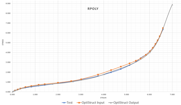
    The RPOLY model correlates well with the test data, and the fit for the material model from test data is good.

  • Ogden Model
    The test data, OptiStruct curve fit and OptiStruct results are plotted.


    Figure 5. Stress-Strain Plot for Ogden Model

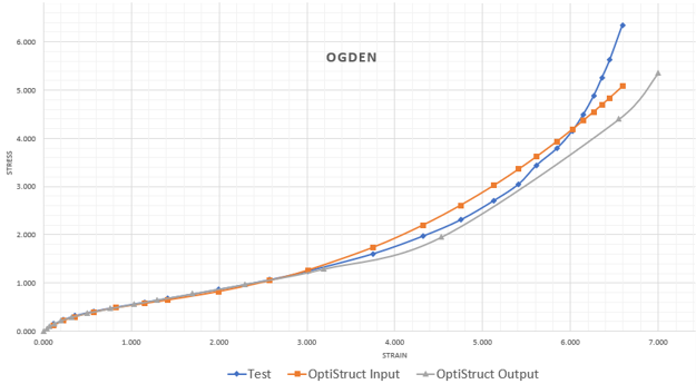
    OptiStruct results and fit correlate well with test data until 300% strain, and continues to be reasonably close beyond 300%.

  • Arruda-Boyce (ABOYCE) Model
    The test data, OptiStruct curve fit and OptiStruct results are plotted.


    Figure 6. Stress-Strain Plot for ABOYCE Model

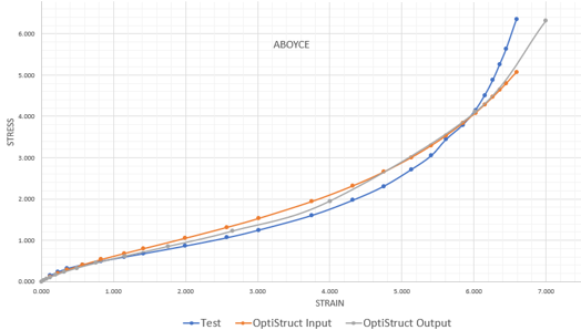
    The ABOYCE model correlates very well with test results until 100% strain and continues to be a reasonably close match beyond 100%.

  • Yeoh Model
    The test data, OptiStruct curve fit and OptiStruct results are plotted. Additionally, Radioss results are illustrated for Yeoh material model.


    Figure 7. Stress-Strain Plot for Yeoh Model

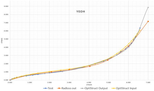
    OptiStruct results correlate well with the test data and fit until about 525% strain and continues to be a reasonably good match beyond 525%. The results obtained by OptiStruct are in good agreement with both test result and Radioss output.

1 Treloar, L. R. G. "Stress-strain data for vulcanised rubber under various types of deformation" Transactions of the Faraday Society 40 (1944): 59-70
2 Miller, Kurt. "Testing Elastomers for Hyperelastic Material Models in Finite Element Analysis" Axel Products, Inc., Ann Arbor, MI (2017). Last modified April 5, 2017

http://www.axelproducts.com/downloads/TestingForHyperelastic.pdf

3 Axel Products, Inc. "Compression or Biaxial Extension?" Ann Arbor, MI (2017). Last modified November 12, 2008

http://www.axelproducts.com/downloads/CompressionOrBiax.pdf