Optimization Problem Setup

During topology optimization, can I use stress constraints through DRESP1 in the design space?

Defining local stress constraints through DRESP1 in the design region for Topology Optimization is allowed. The Stress-Norm method is used to aggregate stress responses.

Can I use the global stress constraint during a topology optimization if I have a mass/volume constraint?

It is not recommended to use the global stress constraint along with a mass/volume constraint. The constrained mass/volume may not allow the stress constraint to be satisfied.

Why are there regions in the model that violate the stress target after running a topology optimization using a global stress constraint?

The stress constraint definition in a topology optimization is a global constraint and does not target local stress concentrations. These areas can be addressed subsequently through size, shape, and free shape optimization or a combination thereof. Artificial stress concentrations are filtered out during topology optimization with stress constraints. These include regions around rigid connections, concentrations due to hard geometric features such as corners, etc.

Why do topology optimizations with global stress constraints not always produce a meaningful result?

Stress constraints may not work well in a model where there is a large differential in response values between design and non-design spaces. In these cases, it is recommended to modify the problem formulation to say, compliance based for example.

Why do I have problems when optimizing a design for its 1st mode frequency?

While targeting first mode frequency, it is recommended that you constrain the first few modes (1-5 for example), as opposed to just the first mode. This results in better stability of the problem and improved convergence. The same applies for buckling responses as well.

After running a topology optimization for a component with four mounting locations, what does it mean when no load path extends to one of the mounting locations?

The reason is that the particular non design part (mounting location) is not needed for the optimal load transfer. If there is a connection to adjacent parts, there should be some loads. Loads will ensure that the region will not be disconnected from the design space.

How do I optimize an aerospace component for cutouts as well as thickness?

It is recommended to optimize for cutouts first through topology optimization, and subsequently for thickness, through free sizing.

Are there any recommendations for running a free size optimization using buckling responses?

While running free-size optimization with buckling responses, it is recommended to use a base thickness value. The optimization process has the tendency to drive the design to simultaneous failure of a large number of buckling modes, potentially as many as the number of design variables. This can only be regulated with a properly chosen base thickness that would prevent formation of an increasing number of local buckling modes.

How can I avoid run termination, due to elements with negative Jacobian during free shape optimization?

Are there any limitations on running topography optimization on a panel while considering an acoustic response? The panel does interface with the fluid domain.

In an acoustic analysis, an interface matrix is calculated between the fluid and structural grids. This interface between the fluid and structural grids is termed the ‘wetted’ surface. Accuracy in calculating this interface is important for determining the accuracy of the solution. While running an optimization, the original interface calculated at the start of the optimization is used throughout the optimization and is not updated during the course of the optimization. As long as the interface is not affected during the optimization, for example, optimizing a component away from the fluid domain, the optimization can be run. However, if during the optimization, the interface is expected to change sufficiently enough through topology, topography or shape for example, the optimization solution may not be accurate. This is based on the implementation as of version 10.0.

Are there any commonly used/suggested topology optimization problem formulations?

Are there any requirements on mesh size for topology optimization?

The density method used for topology optimization is mesh-dependent. It also causes checkerboarding (density value changing rapidly between elements). Models with second order elements do not show this behavior and use of minimum member size constraint treats the checkerboarding issue.

What is the difference between volumefrac response and volume response?

Volumefrac response is the material fraction of the designable material volume. The volume response is the total volume, which includes design and non-design volume.

Is minimizing mass identical to minimizing volume in OptiStruct?

Both formulations are identical as long as the same density r is used for all materials in the model. When minimizing the volume, the density value in the material card does not have to be given.

If different densities r exist in the design and the non-design space, then the optimization result may be different for minimizing mass and minimizing volume.

In a case where the design mass and the non-design mass are almost identical, but the design volume is much smaller than the non-design volume (V_design << V_non-design), minimizing mass will give better results.

On the other hand, when the design volume and the non-design volume are almost identical, but the design mass is much smaller than the non-design mass (r_design << r_non-design), minimizing volume will yield better results.

Is there a way to control the step size of the optimization?

You can change the move limits (the allowable change of the design variable in each iteration step) for the first iteration. The move limits are defined for each optimization type differently. The parameters are DELTOP, DELSHP, DELSIZ on the DOPTPRM statement. They can also be defined for size and shape variables on the DESVAR card.

In HyperMesh, use the Opti Control subpanel in the Optimization panel on the Analysis page.

What is the procedure for restarting an OptiStruct job?

To restart an OptiStruct job, two files are needed: filename.fem (containing input data) and filename.sh (containing design variable information from the end of last complete iteration).

Refer to Requirements for Restarting in the Run OptiStruct section of the documentation.

Is it possible to obtain rib pattern information on shell models using topology optimization?

Yes, but in order to do this, you must define the topology optimization problem differently.

Instead of defining the complete thickness of the shell element as designable, a core non-designable thickness, T0, must be provided in addition to a maximum thickness, T, which includes the core thickness and a designable region (where the ribs can be grown). The topology optimization can then be performed as usual.

The rib patterns can be interpreted by visualization of the density contour plots. Wherever the density values reach 1.0, a rib with the height of the -core plus the designable thickness is needed. Where the density values go to 0.0, no rib is required and it just retains the core thickness.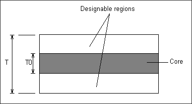

Figure 1.

Example:

Component minimum core thickness: 1.5 mm max thickness with ribs: 3.5 mm

The thickness on the PSHELL card is set to 3.5 mm and T0 on the DTPL card is set to 1.5.

How can I assign and/or change the modweights in a subcase (load case)?

Modeweights are assigned from within a model analysis subcase using the MODEWEIGHT Subcase Information Entry.

From within the HyperMesh panels, access the Optimization panel and the responses subpanel. If the wfreq or comb is chosen as the "response type," you can assign up to six modeweights to six different modes.

How do I calculate the NORM factor for a combined compliance and frequency optimization problem?

If the value of the Subcase Information Entry NORM is left as 0.0 (default), then the normalization factor is estimated during the zero-th (analysis only) iteration of the optimization run (such that the static compliance and weighted frequencies are equally weighted). If you provide a value other than 0.0, that value will be used in the optimization. In HyperMesh, the value of NORM may be defined in the Response panel when the "response type" is comb.

The normalization factor (NORM) is used for normalizing the contributions of static load case compliances and the inverse of eigenvalues when using the combined compliance index as the objective function. A typical structural compliance value is on the order of 1.e4 to 1.e6. However, a typical inverse eigenvalue, as in the case of using the combined compliance index as the objective function, is on the order of 1.e-5. If NF is not used, the linear static compliance requirements dominate the solution. Refer to Responses in the User Guide for more information on the "Combined Compliance Index" and the use of the NORM value.

What is the difference between specifying a constraint on the designable volume and minimizing the designable volume?

In the first method, you can tell OptiStruct to use only a certain fraction of the designable volume (that is, constraining the volume). OptiStruct will redistribute and reorient the amount of the material within the design domain while optimizing the objective function and satisfying any other constraints specified.

In the second method, you can choose their objective to minimize the volume. Here, OptiStruct will minimize the volume to arrive at a final topology that satisfies other constraints.

What is the difference between using forces and prescribed displacements?

In order to increase stiffness, minimize compliance should be used with forces and maximize compliance with prescribed displacements.

The compliance is defined as:

Compliance ~ Force · Displacement

When prescribed displacements are used, the reaction force must be increased to increase the stiffness. This means that the compliance has to be maximized.

In case the forces are given, a stiffer structure means having lower displacements. To achieve this goal, the compliance needs to be minimized.

What is the initial value of material fraction at the beginning of an optimization run (iteration 0)?

If the objective of the design problem is to minimize volume response or mass response, the initial material fraction will be set to 0.9 by default. If a mass or volume constraint is used in the design problem, the initial material fraction will be the value corresponding to the value defined on the constraint. When mass or volume response is not being used to define the objective or the constraint, the material fraction will default to 0.6 at iteration 0.

How can I assign material fraction to 1 at iteration 0?

The initial volume fraction can be assigned to 1.0 (or any other value between 0.0 and 1.0) by defining the MATINIT parameter on the DOPTPRM Bulk Data Entry. This can be done from the HyperMesh interface by changing the value of the MATINIT parameter and checking the corresponding check box in the Opti Control subpanel, under the Optimization panel (located on the Analysis page).

Can I combine various optimization types (size with shape and/or topography)?

Yes, any type of combined optimization can be performed with OptiStruct. It is recommended, however, that different types of optimization be performed separately first. This will help you understand the performance of the structure with different kinds of optimization before attempting a combined optimization.

To set up an optimization problem using more than one optimization type, access the Optimization panel and choose the subpanels for the optimization types to be performed (topology, topography, size and/or shape). If more than one subpanel is chosen in the Optimization panel, (both topology and topography, for example) OptiStruct will automatically perform the combined optimization.

For details on setting up different types of optimization, refer to the OptiStruct tutorials of the documentation.

The results of iteration 0 in an attempted topology optimization are different from the results of a run with ANALYSIS. What is wrong?

Nothing is wrong. You have defined a design space for your topology optimization. In an analysis-only run, the density of the design space is set to 1.0. In the first iteration of the topology optimization, the density of the design space is less than 1.0, unless you have expressly set the MATINIT value, defined on the DOPTPRM Bulk Data Entry, to 1.0. Therefore, in the first iteration, the structure appears to be not as stiff as in an analysis-only run.

For topology optimization runs with mass (volume) as the objective, the default for MATINIT is 0.9. For runs with constrained mass (volume), the default is reset to the constraint value. If mass (volume) is not the objective function and is not constrained, the default is 0.6.

To perform an analysis only run with the modal parameters set to the values that will be used for the first optimization iteration, do not use the ANALYSIS command, and set MAXITER=0.

How can I follow the iteration history while OptiStruct is running?

You can open the iteration history file .hgdata using HyperGraph (or HyperView) while OptiStruct is still running and create plots of the Objective, Constraints, and Design Variables against Iteration. Clicking Apply on the Edit Curves panel, the view can be updated periodically.

Can I use stress constraints with topology or free-size optimization?

• Norm-based Approach (Topology and Free-size Optimization)

  The Norm-based approach is the default method for handling stress responses for Topology and Free-Size Optimization. This method is used when corresponding stress response RTYPE’s on the DRESP1 Bulk Data Entry are input.

  The Response-NORM aggregation is internally used to calculate the stress responses for groups of elements in the model. Solid, shell, bar stresses and solid corner stresses are supported with the Response-Norm aggregation approach (Free-size Optimization is only supported for shell stresses). Refer to NORM Method for more information.

• Augmented Lagrange Method (ALM) (Topology Optimization only)

  The Augmented Lagrange Method (ALM) is an alternative method for handling stress responses for Topology Optimization. It can be activated using DOPTPRM,ALMTOSTR,1 when DRESP1 Bulk Data Entry is used to specify local stress responses.

  ALM is also an alternative method to efficiently solve topology optimization problems with local stress constraints, which is stated in Equation 1.

  $\min f\left(X\right)$ (1)

  $$s.t.g_j\left(X\right)\le 0,j=1,\dots ,m_1$$

  $g_j\left(X\right)\le 0,j=m_1+1,\dots ,m_1$

  Where,

  $X$

  Vector of topology design variables

  $f(X)$

  Objective function

  $g_j\left(X\right)$

  j^th constraint

  $m_1$

  Number of local stress constraints

  $m$

  Total number of constraints

  (2)EQ 2

  $$s.t.g_j\left(X\right)\le 0,j=m_1+1,\dots ,m_1$$
  Where,

  $h_j\left(X\right)=max\left[g_j\left(X\right),-\frac{{\lambda }_j}{\mu }\right]$

  $g_j\left(X\right)=E_j\left(\frac{{\sigma }_j}{{\sigma }_{lim}}-1\right)\left[1+{\left(\frac{{\sigma }_j}{{\sigma }_{lim}}-1\right)}^2\right]$

  $, j=1,\dots ,m_1$

  $E_j=\epsilon +\left(1-\epsilon \right){\left[\frac{tanh\left(\beta \eta \right)+tanh\left(\beta \left({\rho }_j-\eta \right)\right)}{tanh\left(\beta \eta \right)+tanh\left(\beta \left(1-\eta \right)\right)}\right]}^p$

  ${\rho }_j$

  Element density

  ${\sigma }_j$

  Element von Mises stress

  ${\sigma }_{\lim }$

  stress upper bound

  ${\lambda }_j$

  Lagrange multiplier estimator

  $\mu >0$

  Quadratic penalty factor

  The penalty factor is typically updated as:(3)

  $${\mu }^{\left(k+1\right)}=min\left(\alpha {\mu }^{\left(k\right)},{\mu }_{max}\right)$$

  Where,

  $\alpha >1$

  Update parameter

  ${\mu }_{\max }$

  Upper limit to prevent numerical instabilities

  (4)
  $${\mu }^{\left(k+1\right)}=min\left(\alpha {\mu }^{\left(k\right)},{\mu }_{max}\right)$$

  The Lagrange multiplier estimators are updated as ${\lambda }_j^{\left(k+1\right)}={\lambda }_j^{\left(k\right)}+{\mu }^{\left(k\right)}{h}_j\left(X\right)$ .

  In general, the number of local stress constraints $m_1$ is very large. Directly solving Equation 1 is computationally time consuming. By penalizing the stress constraints onto the objective function, the total number of constraints can be significantly reduced. As a result, the optimization problem can be efficiently solved.

  The parameters are set as ${\mu }^{(0)}=10$ , ${\mu }_{\max }={10}^6$ , $\alpha =1.3$ , $\eta =0.5$ , $\epsilon ={10}^{-6}$ , $p=3$ . $\beta$ is initially set to 1.0 and multiplied by 1.3 in every five iterations, with an upper limit of 30.0. Based on this process, Topology Optimization is carried out within one phase.

  Note: Except for this ALM, OptiStruct generally uses a multi-phase strategy to solve topology optimization problems.

  The default Stress-norm (P-norm) method continues to efficiently solve Topology Optimization problems with local stress constraints. The ALM ¹ is a good alternative for such models.

• Global von Mises Stress Response (Topology and Free-size Optimization)
  The von Mises stress constraints may be defined for topology and free-size optimization through the STRESS optional continuation line on the DTPL or the DSIZE card. There are a number of restrictions with this constraint:

  • The definition of stress constraints is limited to a single von Mises permissible stress. The phenomenon of singular topology is pronounced when different materials with different permissible stresses exist in a structure. Singular topology refers to the problem associated with the conditional nature of stress constraints, that is, the stress constraint of an element disappears when the element vanishes. This creates another problem in that a huge number of reduced problems exist with solutions that cannot usually be found by a gradient-based optimizer in the full design space.
  • Stress constraints for a partial domain of the structure are not allowed because they often create an ill-posed optimization problem since elimination of the partial domain would remove all stress constraints. Consequently, the stress constraint applies to the entire model when active, including both design and non-design regions, and stress constraint settings must be identical for all DSIZE and DTPL cards.
  • The capability has built-in intelligence to filter out artificial stress concentrations around point loads and point boundary conditions. Stress concentrations due to boundary geometry are also filtered to some extent as they can be improved more effectively with local shape optimization.
  • Due to the large number of elements with active stress constraints, no element stress report is given in the table of retained constraints in the .out file. The iterative history of the stress state of the model can be viewed in HyperView or HyperMesh.
  • Stress constraints do not apply to 1D elements.
  • Stress constraints may not be used when enforced displacements are present in the model.

  The buckling factor can be constrained for shell topology optimization problems with a base thickness not equal to zero. Constraints on the buckling factor are not allowed in any other cases of topology optimization.

  The following responses are currently available as the objective or as constraint functions for elements that do not form part of the design space:

  Composite Stress	Composite Strain	Composite Failure Criterion
  Frequency Response Stress	Frequency Response Strain	Frequency Response Force

Can I use buckling constraints on a topology or free-size optimization?

Because of the above reasons, for the time being, reasonable success can only be expected for one class of design problems -- shell structures with non-zero base thickness.

Is there a way to find the rigid body modes in a model?

In order to find the rigid body modes, you can add a diagnostic command OSDIAG,46,1 to the I/O Options or Subcase Information sections of the OptiStruct deck. The diagnostic command will output the DOFs that are constrained and provide the rigid body mode results to the user.

Can volume or mass be defined as a response for topography optimization?

The sensitivities of volume are so low for topography optimization that they do not make a significant contribution toward the optimization. It is recommended that using both volume and mass as responses be avoided

How can the same response from different loadsteps be added together?

This can be achieved through the use of DEQATN, DRESP2, and DRESP1L cards. A DEQATN is defined to sum a number or responses. This DEQATN is referenced on a DRESP2 definition, which uses the DRESP1L continuation to select the same DRESP1 response for a number of different subcases.

Within HyperMesh, this can be achieved by first defining a dequation. Then, in the Response panel, select function as the response type, select the already-defined dequation, click edit, select Responses_by_loadstep from the available options, and select the same response for a number of different loadsteps.

$
$  OBJECTIVES Data
$
$
$HMNAME OBJECTIVES       2objective
$
DESOBJ(MIN)=5
$
$
DESGLB        9
$
$
$HMNAME LOADSTEPS       1brake
$
SUBCASE       1
 SPC  =       1
 LOAD =       2
$
$HMNAME LOADSTEPS       2corner
$
SUBCASE       2
 SPC  =       1
 LOAD =       3
$
$HMNAME LOADSTEPS       3pothole
$
SUBCASE       3
 SPC  =       1
 LOAD =       4
$
BEGIN BULK

$HMNAME DESVARS        1topo_arm
$TPL    1       0.0     0.0     1       1       14
$
$  OPTIRESPONSES Data
$
DRESP1  3       comp    COMP    PSOLID                                14
DRESP2  5       wcomp          1
+       DRESP1L        3       1       3       2       3       3
DRESP1  9       vol     VOLFRAC
$
$HMNAME DEQUATIONS       1eq1
$
DEQATN  1       f(a,b,c)=a+b+c
$
$
$  OPTICONSTRAINTS Data
$
$
$HMNAME OPTICONSTRAINTS       8vol
$
DCONSTR        8       9        0.1
DCONADD        9       8