
Absolute Nodal Coordinate Formulation
The Absolute Nodal Coordinate Formulation or the ANCF is a finite element based representation of flexible components in one, two and three dimensions that are allowed to deform under applied load. It is a formulation that allows you to model Non Linear Flexible Element (NLFE) components in your multibody system.
Such flexible components can be used to describe the dynamic motion of deformable bodies. Owing its fully non-linear formulation, this method is capable of handling large deformation as well as large rotation within its elements. The ANCF as implemented in MotionSolve also allows you to model materials with non-linear characteristics like rubber and other hyper-elastic materials.
BEAM Elements
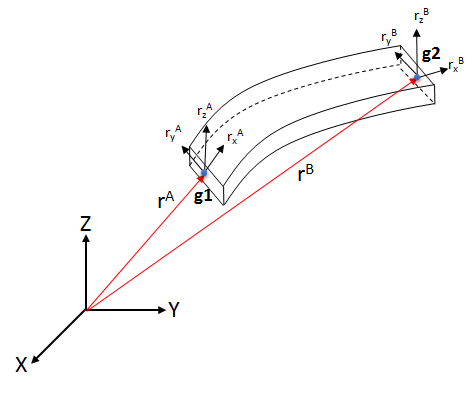
- Position of the grid in 3D space
-
- Gradient vector in X direction
- Gradient vector in Y direction
- Gradient vector in Z direction
- Defines the axial strain in the X direction
- Defines the axial strain in the Y direction
- Defines the axial strain in the Z direction
- Degree of Freedom of the Grid
- Rigid translation of the grid along X axis
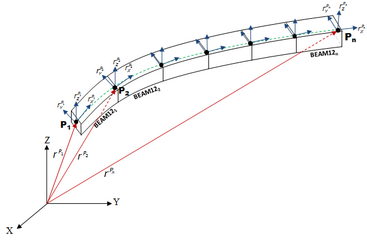
The geometric properties of the BEAM12 element can be specified using the PBEAML element which lets you define the cross section of the beam along with the relevant dimensions. In addition to the geometric properties, you also need to specify material properties for the BEAM12 element. The BEAM 12 element supports linear elastic and hyper-elastic models that define the material model. For more information, please refer to the different material property elements in the documentation.
CABLE Elements
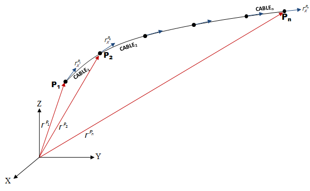
The second type of LINE element supported in MotionSolve is the CABLE element. Such a CABLE element can be considered a LINE element in that it is defined by two nodes - one at the start (g1) and one at the end (g2) of the element. This is illustrated in Figure 3.
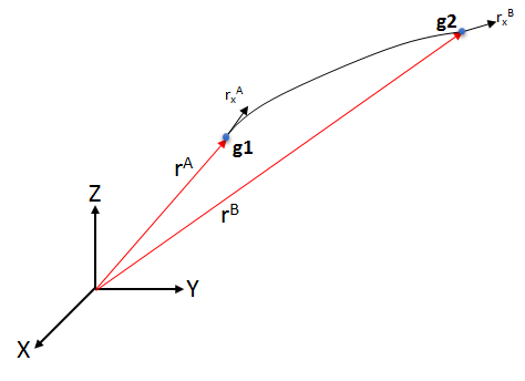
- Position of the grid in 3D space
- Gradient vector in X direction
- Defines the axial strain in the X direction
Based on the construction of this element, it is easy to see that it can only resist axial and bending loads. The cross section of this element is assumed to be constant and does not deform with increasing load.
- Degree of Freedom of the Grid
- Rigid translation of the grid along X axis
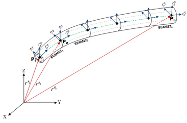
A wire or cable component can thus be modeled using multiple CABLE elements as shown in Figure 4.
The geometric properties of the CABLE element can be specified using the PCABLE element which lets you define the cable cross section area, moment of area and other post processing flags. In addition to the geometric properties, you also need to specify material properties for the CABLE element. The CABLE element supports only the linear elastic material model. For more information, please refer to the documentation.
Specify Materials for BEAM and CABLE Elements
- Material Type
- Element Type
- Linear elastic (Continuum mechanics and elastic line approach).
- BEAM12 and CABLE
- Hyper elastic (Neo-Hookean, Mooney Rivlin and Yeoh).
- BEAM12 only
- The material deforms in a reversible fashion. That is, as soon as the load is removed, it returns to its original shape
- The stress is a linear function of strain
- The strain is not dependent on the loading rate
The linear elastic material model is defined by three parameters - the Young's modulus, Poisson's ratio and the density of the material. This model can be used to model most metals and plastics up until a threshold load beyond which they will start to exhibit plastic deformation and finally yield.
Values for these three material parameters are typically obtained by testing the material in a laboratory. However, owing to the simplicity of this material model, these values are sometimes readily available in textbooks and in engineering handbooks.
- The stress in the material is not a linear function of the strain
- This type of material model is used to model large strains as high as 200%
Hyper-elastic material models are typically used to model elastomers (like rubber), polymers, foams, biological materials (like muscle) etc. To model such a material, constitutive laws are used which make use of the strain energy density functions. The strain energy density can be thought of the area under the stress-strain curve for any material. For more information on the formulation of the strain energy density function, please refer to the reference manual.
- Type of Material Law
- Parameters Used to Define the Material
- Neo-Hookean material law
- (Shear modulus) and density
- Mooney-Rivlin material law
- (Material constant)
- Yeoh material law
- (Material constant)
While the Shear modulus, Poisson's ratio and density parameters may be available in engineering handbooks or textbooks, the material constants for the Mooney-Rivlin and Yeoh material law are determined through lab testing. Typically, uniaxial, biaxial and planar tests are conducted to measure the stresses and strains in the material at different operating points. A curve is then fitted through this data which represents the non-linear relationship between stress and strain. A typical stress-strain relationship for these three material laws is illustrated in Figure 5 obtained through a uni-axial test.

Which material model should I use?
Depending on the application and the expected strain in the hyper-elastic material, the choice of material laws changes. For applications where a low strain (<10%) is expected, it may be satisfactory to use a linear elastic material. If you are expecting larger strains (for example, while modeling rubber), it is recommended to start with the Neo-Hookean model that is the simplest of the three hyper-elastic models.
If test data is readily available, either the Yeoh or the Mooney-Rivlin model may be used. The choice of which model to use between these two depends on how good of a curve fit is obtained between the material laws and the test data over the range of the strain/stretch that is desired.
MotionView provides a sample set of coefficient values for all three hyper-elastic material models. You may also use your own material constants in MotionView.