ACU-T: 6500 Flow Through Porous Medium

Prerequisites

This tutorial provides the instructions for setting up, solving and viewing results for a simulation of a flow through porous medium. Prior to starting this tutorial, you should have already run through the introductory tutorial, ACU-T: 1000 Basic Flow Set Up, and have a basic understanding of HyperMesh CFD and AcuSolve. To run this simulation, you will need access to a licensed version of HyperMesh CFD and AcuSolve.

Before you begin, copy the file(s) used in this tutorial to your working directory.

ACU-T6500_PorousMedia.hm

Problem Description

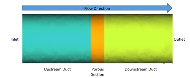
The problem to be addressed in this tutorial is shown schematically in the figure below. It consists of a cylindrical channel with a porous medium in the flow section. As the flow passes through this section, a pressure drop is observed. In this simulation, an inlet velocity will be assigned to the flow and pressure drop across the porous medium will be calculated. The length of the porous section is 0.06 m and the fluid is air with a density of 1.225 kg/m³ and a molecular viscosity of 1.781e-5 kg/m-s. The inlet velocity of the flow is 0.2 m/s.

In AcuSolve, a porous media problem can be solved using one of two methods: the superficial velocity method and physical velocity method. In this tutorial, we adopt the superficial velocity method, which provides good representation of the pressure drop through a porous media. However, it cannot predict the velocity increase in the porous region since the velocity in the porous region remains the same as those outside of the porous zones. The more accurate representation of velocity inside the porous region can be obtained using the physical velocity method, which solves the continuity and momentum equation inside the porous media using the intrinsic averaging method.

The pressure loss across the porous region using the superficial velocity method is modelled as:

\frac{Δ P}{Δ x_{i}} = C_{D} \frac{μ}{k} V_{i} + C_{p} \frac{ρ}{\sqrt{k}} V_{m} V_{i}

where $Δ P$ is the pressure drop (Pa) across the porous region, $Δ x_{i}$ is the porous region length (m), $k$ is the permeability, $C_{D}$ is the Darcy coefficient, $C_{p}$ is the Forchheimer coefficient, $μ$ is the viscosity (kg/m-sec), $ρ$ is density (kg/m³), $V_{m}$ is velocity magnitude (m/sec), and $V_{i}$ is velocity (m/sec).

In this tutorial, you will utilize the porous coefficient calculator to calculate the Darcy coefficient and the Forchheimer coefficient after curve fitting of the array data of pressure drop vs velocity. The pressure drop across the porous region can be simplified as the permeability is not included in the curve fitting.

\frac{Δ P}{Δ x} = C_{D} μ V_{x} + C_{p} ρ V_{x}^{2} \sim B V_{x} + A V_{x}^{2}

The figure below shows the Darcy and Forchheimer coefficient calculator after providing the velocity (m/s) and pressure drop (Pa) data in addition to the thickness (m) of the porous medium zone, density (kg/m³) and viscosity (kg/m-s) of air.

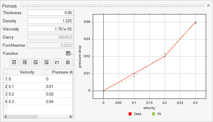
The Darcy coefficient $C_{D}$ and Forchheimer coefficient $C_{p}$ are then calculated based on the curve fit coefficients

Start HyperMesh CFD and Open the HyperMesh Database

Start HyperMesh CFD from the Windows Start menu by clicking Start > Altair <version> > HyperMesh CFD.
From the Home tools, Files tool group, click the Open Model tool.

Figure 3.

The Open File dialog opens.
Browse to the directory where you saved the model file. Select the HyperMesh file ACU-T6500_PorousMedia.hm and click Open.
Click File > Save As.
Create a new directory named PorousMedia and navigate into this directory.
This will be the working directory and all the files related to the simulation will be stored in this location.
Enter PorousMedia as the file name for the database, or choose any name of your preference.
Click Save to create the database.

Validate the Geometry

The Validate tool scans through the entire model, performs checks on the surfaces and solids, and flags any defects in the geometry, such as free edges, closed shells, intersections, duplicates, and slivers.

To focus on the physics part of the simulation, this tutorial input file contains geometry which has already been validated. Observe that a blue check mark appears on the top-left corner of the Validate icon on the Geometry ribbon. This indicates that the geometry is valid, and you can go to the flow set up.

Set Up Flow

Set Up the Simulation Parameters and Solver Settings

From the Flow ribbon, click the Physics tool.

Figure 5.

The Setup dialog opens.
Under the Physics models setting:
1. Set Time marching to Steady.
2. Select Laminar as the Turbulence model.
Figure 6.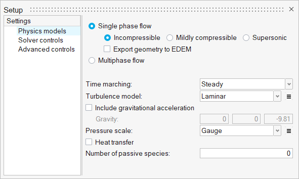
Click the Solver controls setting.
Confirm that the Steady update factor and the Steady maximum steps are set to 0.6 and 100, respectively.

Figure 7.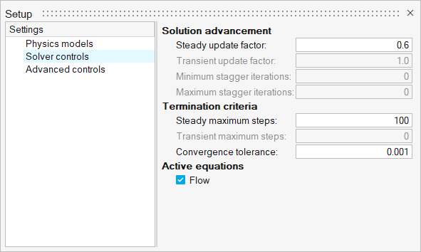

Assign Material Properties

From the Flow ribbon, click the Material tool.

Figure 8.
Verify that the material Air is assigned to the model's three solids.

Figure 9.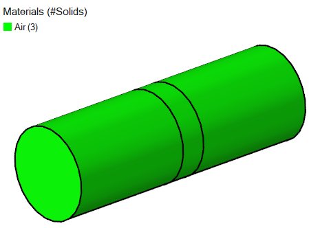

Define the Porous Medium

From the Flow ribbon, Porous tool group, click the Cartesian Porous Media tool.

Figure 10.
Select the middle solid on the model.

Figure 11.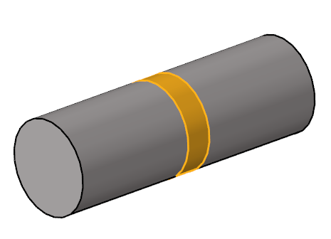
On the guide bar, click Orientation.
Left-click to place a point anywhere on the selected solid.
In the microdialog, click the coefficient calculator and enter the following values for the coefficient calculator.
- porous zone thickness = 0.06 (m)
- air density = 1.225 kg/m³
- air viscosity = 1.781e-05 kg/m-sec
Figure 12.
Close the coefficient calculator and confirm the values of the Darcy coefficient and Forchheimer coefficient. Enter permeability values for the three directions as shown in the figure below

Figure 13.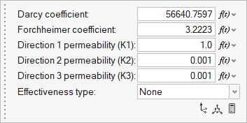
In the microdialog, click to open the Orient tool then verify that the direction is aligned to the global x-axis.

Figure 14.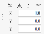
On the guide bar, click to execute the command and exit the tool.

Assign the Flow Boundary Conditions

From the Flow ribbon, click the Constant tool.

Figure 15.
Select the inlet face.

Figure 16.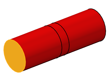
In the microdialog, set the velocity parameters as shown below.

Figure 17.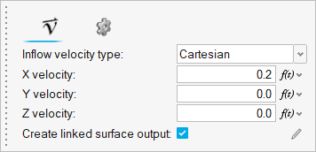
On the guide bar, click to execute the command and exit the tool.
Click the Outlet tool.

Figure 18.
Select the outlet face.

Figure 19.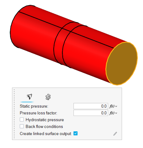
Accept the default parameters then click on the guide bar.

Generate the Mesh

The meshing parameters for this tutorial are already set in the input file.

From the Mesh ribbon, click the Volume tool.

Figure 20.

The Meshing Operations dialog opens.
Note: If the model has not been validated, you are prompted to create the simulation model before running the batch mesh.
Check that the Average element size is 0.01.
Accept all other default parameters.

Figure 21.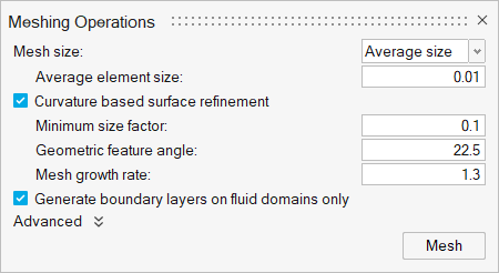
Click Mesh.
The Run Status dialog opens. Once the run is complete, the status is updated and you can close the dialog.
Tip: Right-click on the mesh job and select View log file to view a summary of the meshing process.

Run AcuSolve

From the Solution ribbon, click the Run tool.

Figure 22.
Set the Parallel processing option to Intel MPI.
Optional: Set the number of processors to 4 or 8 based on availability.
Leave the remaining options as default and click Run to launch AcuSolve.

Figure 23.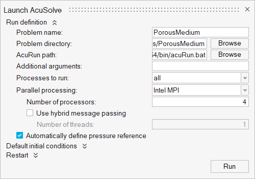

Post-Process with the Plot Tool

In the Run Status dialog, right-click on AcuSolve run and select Plot time history to launch the Plot Manager.

Figure 24.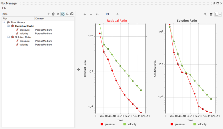
Click to create a new plot.
Click under the Model panel to create a user defined function.
In the Data Tree, expand Integrated Surface Output > Pressure then select pressure.
In the Name field, enter dP.
In the Value field, type value=.
Under Parts, choose AUTO Porous-1 SolidBody_2_1 internal then click Insert Field to insert the field as part of the value, as shown below.

Figure 25.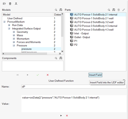
Type - at the end of the user defined function value.
Under Parts, choose AUTO Porous-3 SolidBody_4_3 internal then click Insert Field to insert the field as part of the value.
Click to add the user defined function.

Figure 26.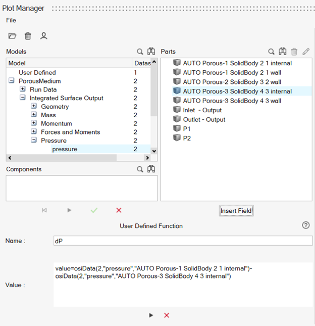
Click the x axis to switch to Time Steps.

Figure 27.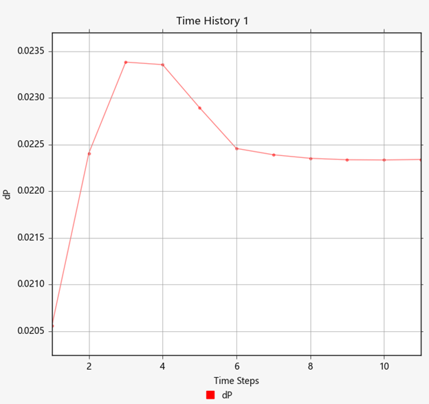

The pressure drop across the porous inlet (AUTO Porous-1 SolidBody_2_1 internal) and porous outlet (AUTO Porous-3 SolidBody_4_3 internal) surfaces is 0.0223 Pa.

Summary

In this tutorial, you learned how to set up and solve a flow simulation with porous medium. You started by importing the HyperMesh CFD input database and then you defined the porous medium. You also learned how to compute the Darcy and Forchheimer coefficients using the calculator available in HyperMesh CFD. Next, you assigned the flow boundary conditions and generated the mesh. Once the solution was computed, you created a plot of the pressure drop across the porous section using the Plot tool.