
ACU-T: 4003 Freely Falling Water Droplet
Tutorial Level: Intermediate
Prerequisites
This tutorial introduces you to the workflow for setting up a transient droplet simulation using HyperMesh CFD. Prior to starting this tutorial, you should have already run through the introductory tutorial, ACU-T: 1000 Basic Flow Set Up, and have a basic understanding of HyperMesh CFD and AcuSolve. To run this simulation, you will need access to a licensed version of HyperMesh CFD and AcuSolve.
Problem Description
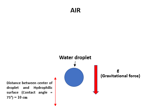
Start HyperMesh CFD and Open the HyperMesh Database
- Start HyperMesh CFD from the Windows Start menu by clicking .
-
From the Home tools, Files tool group, click the Open Model tool.
Figure 2. 
The Open File dialog opens. - Browse to the directory where you saved the model file. Select the HyperMesh file ACU-T4003_FallingDroplet.hm and click Open.
- Click .
-
Create a new directory named ContactAngle and navigate into this directory.
This will be the working directory and all the files related to the simulation will be stored in this location.
- Enter FallingDroplet as the file name for the database, or choose any name of your preference.
- Click Save to create the database.
Validate the Geometry
The Validate tool scans through the entire model, performs checks on the surfaces and solids, and flags any defects in the geometry, such as free edges, closed shells, intersections, duplicates, and slivers.
Set Up Flow
Create Materials
-
From the Flow ribbon, click the Material Library tool.
Figure 4. 
The Material Library dialog opens. - Under Settings, click Immiscible Multiphase and then click the My Materials tab.
-
Click
 to create a new material.
-
In the new dialog, rename the material to air_water_st
by clicking the name in the top-left corner, then enter the properties shown
below.
Figure 5. 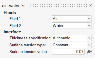
Set Up the Simulation Parameters and Solver Settings
-
From the Flow ribbon, click the Physics tool.
Figure 6. 
The Setup dialog opens. -
Under the Physics models setting:
- Activate the Multiphase flow radio button.
- Set the Multifluid type to Immiscible and the Immiscible material to air_water_st.
- Set the Time step size to 0.0005 and the Final time to 0.15.
- Select Laminar as the Turbulence model.
- Set the gravity to -9.81 m/sec2 in the y direction.
Figure 7. 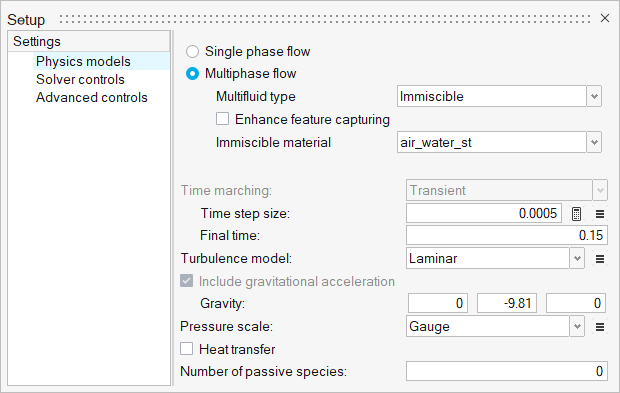
-
Click Solver controls and verify the following:
- Minimum stagger iterations: 0
- Maximum stagger iterations: 6
- The Flow and Multifluid checkboxes are activated.
Figure 8. 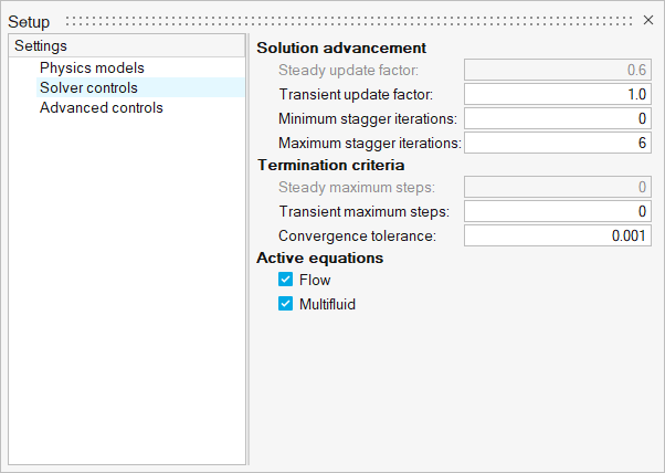
- Close the dialog and save the model.
Assign Material Properties
-
From the Flow ribbon, click the Material tool.
Figure 9. 
- Verify that air_water_st has been assigned to the volume.
-
Click
 on the guide bar.
Define Flow Boundary Conditions
-
From the Flow ribbon, click the Symmetry tool.
Figure 10. 
-
Click
 on the View Controls toolbar and
set the model orientation to Isometric.
on the View Controls toolbar and
set the model orientation to Isometric.
-
Select the Z-Positive face, as highlighted below.
Figure 11. 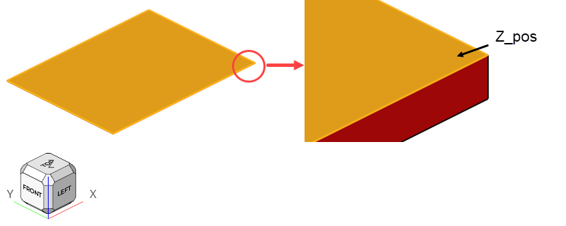
- In the Boundaries legend, double-click Symmetry and rename it to Z_pos.
-
On the guide bar, click
 to execute the command and remain in the
tool.
to execute the command and remain in the
tool.
- Rotate the model and select the opposite face.
- In the Boundaries legend, double-click Symmetry and rename it to Z_neg.
-
On the guide bar, click
 to execute
the command and exit the tool.
to execute
the command and exit the tool.
-
Click the Outlet tool.
Figure 12. 
- In the Boundaries legend, right-click Default Wall and select Isolate.
-
Click on the View Controls toolbar and
set the model orientation to Isometric.
-
Select the top and side faces, as highlighted below.
Figure 13. 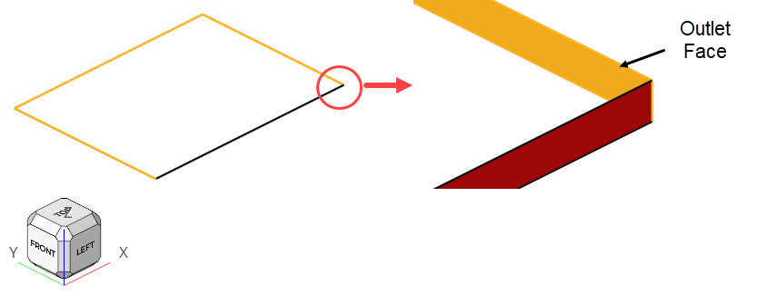
-
In the microdialog, set the following properties and
then click on the guide bar.
Figure 14. 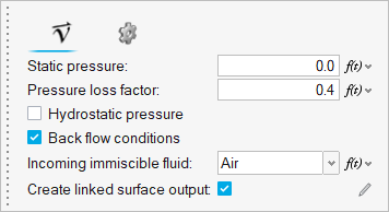
-
Click the No Slip tool.
Figure 15. 
- In the Boundaries legend, Isolate the Default Wall then Show the Outlet faces.
-
Select the face highlighted below.
Figure 16. 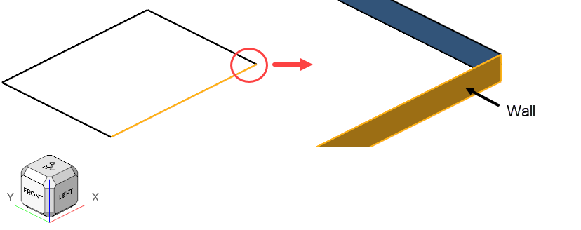
-
In the microdialog, activate the Specify
contact angle checkbox, set the Contact angle value to
75, and then click on the
guide bar.
Figure 17. 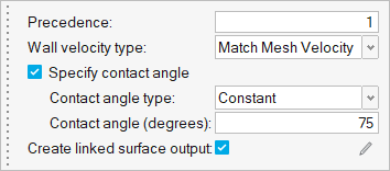
Generate the Mesh
-
From the Mesh ribbon, click the
Volume tool.
Figure 18. 
The Meshing Operations dialog opens. - Check that the Average element size is 0.006.
-
Accept all other default parameters.
Figure 19. 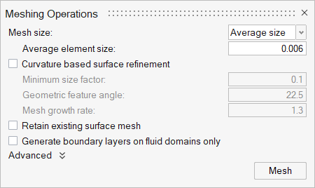
-
Click Mesh.
The Run Status dialog opens. Once the run is complete, the status is updated and you can close the dialog.Tip: Right-click the mesh job and select View log file to view a summary of the meshing process.
Define Nodal Outputs and Nodal Initial Conditions
In this step, you will define the nodal output frequency and then specify the nodal initial conditions for the water droplet.
Define Nodal Output Frequency
-
From the Solution ribbon, click the Field tool.
Figure 20. 
The Field Output dialog opens. - Click the Solution variables setting.
- Activate the Write initial conditions checkbox.
-
Verify that the Write results at time step interval
checkbox is active.
Figure 21. 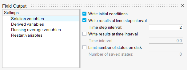
Define Nodal Initial Conditions
-
From the Solution ribbon, Zones tool group, click the Cylinder tool.
Figure 22. 
- Select the Top face on the View Cube to orient the model.
-
Double-click the geometry to create the cylinder-shaped zone and then press
Esc.
Figure 23. 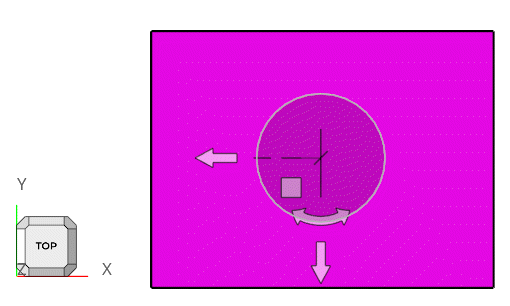
- To provide the dimensions of the cylinder, right-click Nodal initial condition cylinder in the legend and select Edit.
-
In the microdialog, click the icon on the right to
expand the menu, and then set the radius to 0.001 and the
height to 0.00339589.
Figure 24. 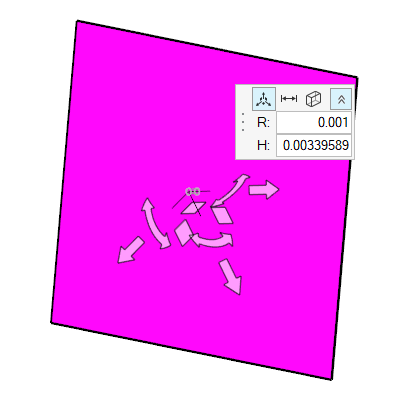
-
Click on the View Controls toolbar and
select Isometric.
Figure 25. 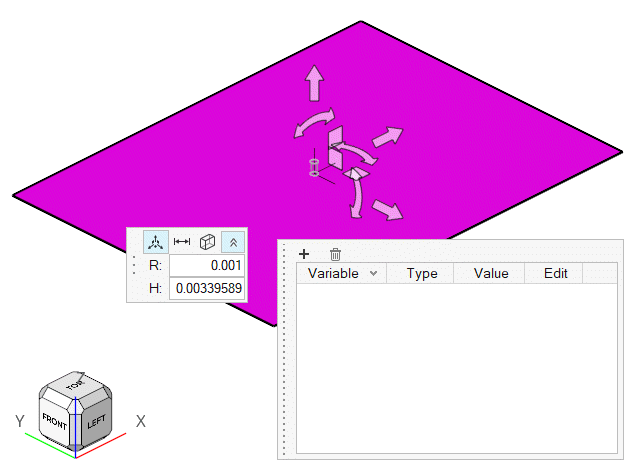
-
Zoom in on the zone and select the base point of the cylinder, as shown in the
figure below. Set the coordinates to (0.06, 0.02,
-0.001).
Figure 26. 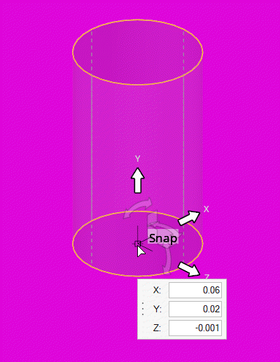
-
Select the Rear face on the View Cube and verify that
cylinder zone is passing over the domain completely as shown in the figure
below.
Figure 27. 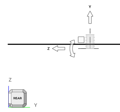
-
In the initial condition dialog, click , select
Fluid, and then left-click in empty space.
-
Change the fluid to Water.
Figure 28. 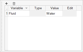
Run AcuSolve
-
From the Solution ribbon, click the Run tool.
Figure 29. 
- Set the Parallel processing option to Intel MPI.
- Optional: Set the number of processors to 4 or 8 based on availability.
-
Leave the remaining options as default and click
Run to launch AcuSolve.
Figure 30. 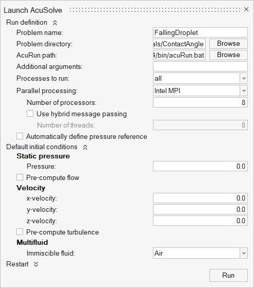
The Run Status dialog opens. Once the run is complete, the status is updated and you can close the dialog.Tip: While AcuSolve is running, right-click the AcuSolve job in the Run Status dialog and select View Log File to monitor the solution process.
Post-Process the Results with HM-CFD Post
- Once the solution is completed, navigate to the Post ribbon.
- From the menu bar, click .
-
Select the AcuSolve
.log file in your problem
directory to load the results for post-processing.
The solid and all the surfaces are loaded in the Post Browser.
Figure 31. 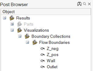
- To check the contours of volume fraction of water on the solid, right-click Z_pos in the Post Browser and select Isolate.
-
Right-click Z_pos again and select
Edit.
A microdialog for surface coloring opens.
- Set the display to volume fraction water and toggle on the Legend radio button.
-
Click
 in the same dialog to verify the legend properties
shown below.
You will be able to see the contours of volume fraction of water at time step=1.
in the same dialog to verify the legend properties
shown below.
You will be able to see the contours of volume fraction of water at time step=1.Figure 32. 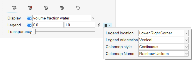
Figure 33. 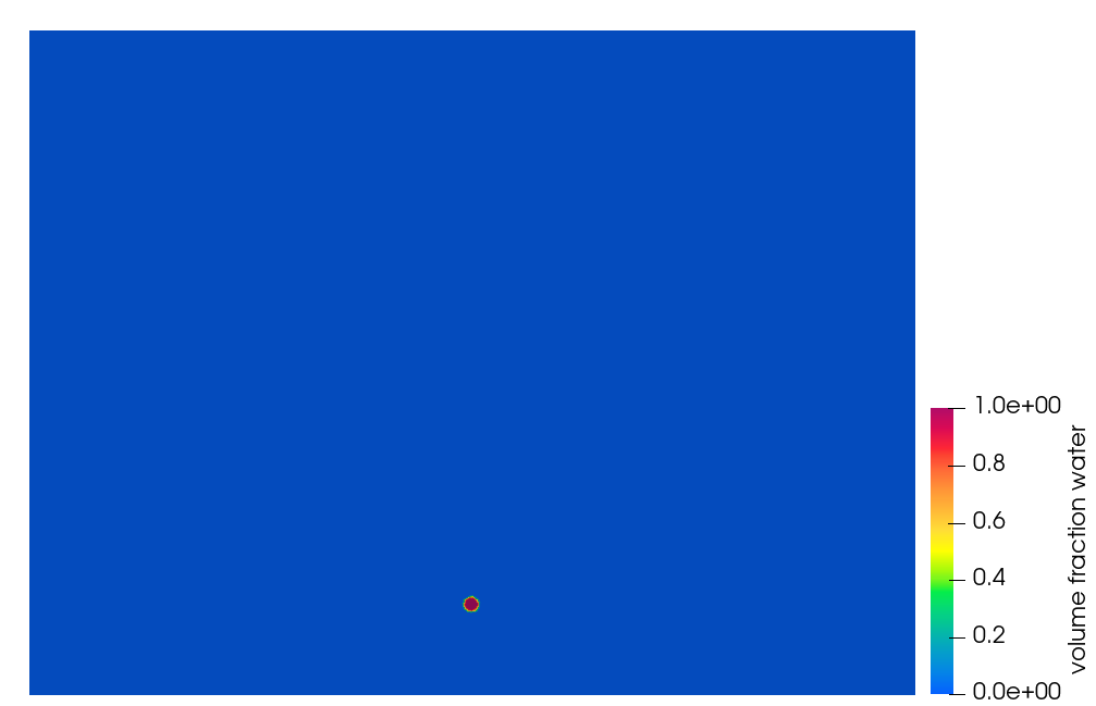
-
Make sure the time scale at the bottom of the modeling window is at time step =1. Click the bar to see the
falling of droplet and interaction of it with surface at time step = 65, 75, 85
and final time step (where 1 time step = 2 secs).
Figure 34. 
Figure 35. 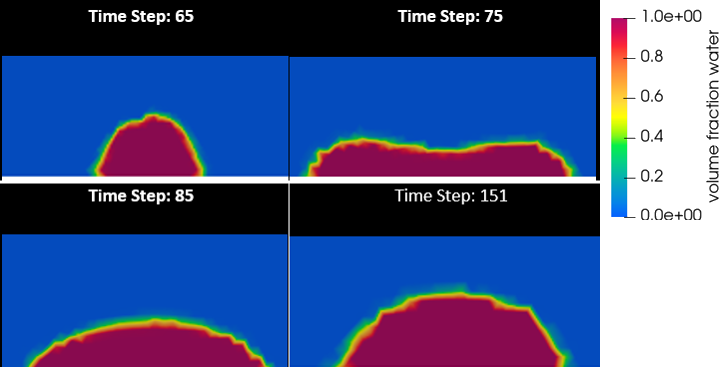
Summary
In this tutorial, you successfully learned how to set up and solve a simulation involving contact angle and surface tension using HyperMesh CFD. You imported the geometry and then defined the simulation parameters and flow boundary conditions. Once the solution was computed, you used HyperMesh CFD Post to create the contours of volume fraction of water.