
ACU-T: 4100 Multiphase Flow using Algebraic Eulerian Model
Tutorial Level: Beginner
This tutorial provides instructions for running a transient simulation of a two-phase flow in a pipe using the Algebraic Eulerian model. Prior to starting this tutorial, you should have already run through the introductory tutorial, ACU-T: 1000 Basic Flow Set Up, and have a basic understanding of HyperMesh CFD and AcuSolve. To run this simulation, you will need access to a licensed version of HyperMesh CFD and AcuSolve.
Problem Description
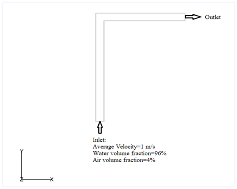
The problem to be addressed in this tutorial is shown schematically in Figure 1. The Algebraic Eulerian (AE) model is used to simulate the momentum exchange between a carrier field and a dispersed field. When simulating multiphase flows using the AE model, the carrier field has to be a heavier fluid (or higher density fluid).
In this problem, Water is considered a Carrier field material and Air is considered as Dispersed field material. Fluid enters the Inlet at an Average Velocity of 1 m/sec and the Water and Air volume fractions at the inlet are 96% and 4% respectively.
Start HyperMesh CFD and Open the HyperMesh Database
- Start HyperMesh CFD from the Windows Start menu by clicking .
-
From the Home tools, Files tool group, click the Open Model tool.
Figure 2. 
The Open File dialog opens. - Browse to the directory where you saved the model file. Select the HyperMesh file ACU-T4100_LPipe.hm and click Open.
- Click .
-
Create a new directory named Algebraic_Eulerian and navigate into this directory.
This will be the working directory and all the files related to the simulation will be stored in this location.
- Enter LPipe_Disperse as the file name for the database, or choose any name of your preference.
- Click Save to create the database.
Validate the Geometry
The Validate tool scans through the entire model, performs checks on the surfaces and solids, and flags any defects in the geometry, such as free edges, closed shells, intersections, duplicates, and slivers.
Set Up Flow
Create Materials
-
From the Flow ribbon, click the Material Library tool.
Figure 4. 
The Material Library dialog opens. - Under Settings, click Disperse Multiphase, and then click the My Materials tab.
-
Click
 to create a new material.
-
Name the material Air in Water and assign the properties
shown below.
Figure 5. 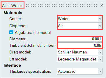
Set the General Simulation Parameters
-
From the Flow ribbon, click the Physics tool.
Figure 6. 
The Setup dialog opens. -
Under the Physics models setting:
- Activate the Multiphase flow radio button.
- Set the Multifluid type to Disperse and the Disperse material to Air in Water
- Set the Time step size to 0.01.
- Select Spalart-Allmaras as the Turbulence model.
- Set the gravity to -9.81 m/sec2 in the y direction.
Figure 7. 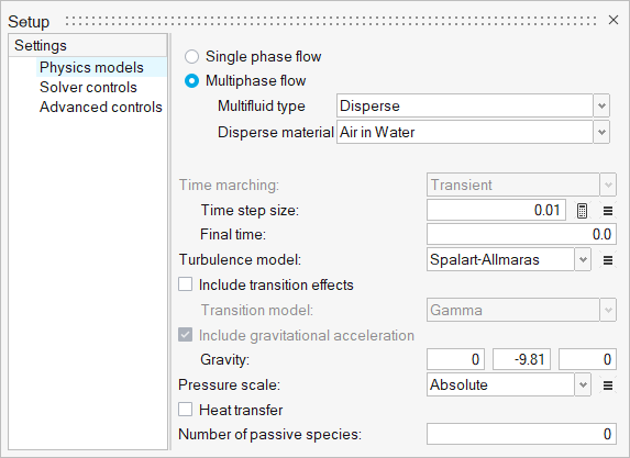
-
Click the Solver controls setting and verify that:
- Minimum stagger iteration is set to 2.
- Maximum stagger iteration is set to 4.
- Transient maximum step is set to 150.
- The Flow, Multifluid, and Turbulence checkboxes are activated.
Figure 8. 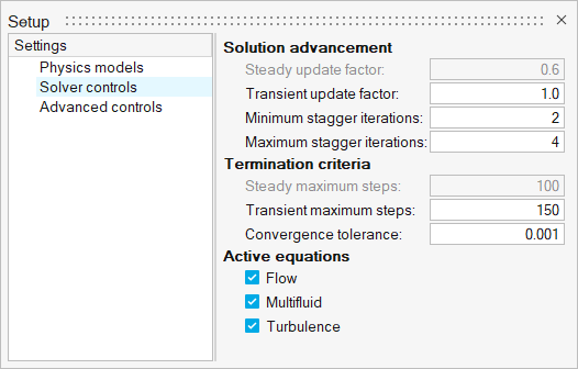
- Close the dialog and save the model.
Assign Material Properties
-
From the Flow ribbon, click the Material tool.
Figure 9. 
- Select the model solid.
-
Select Air in Water from the Material drop-down
menu.
Figure 10. 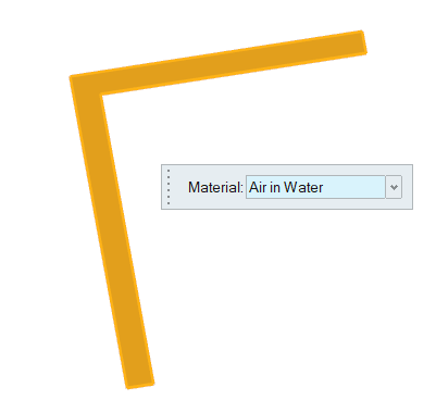
-
On the guide bar, click
 to execute
the command and exit the tool.
to execute
the command and exit the tool.
Define Flow Boundary Conditions
-
From the Flow ribbon, Profiled
tool group, click the Profiled Inlet tool.
Figure 11. 
-
Click the inlet face, highlighted in the figure below.
Figure 12. 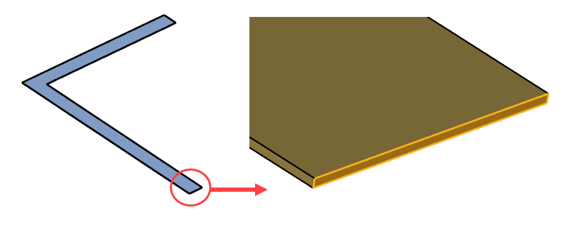
-
In the microdialog, enter 1.0
for the Average velocity and 0.96 for the Carrier fluid
volume fraction.
Figure 13. 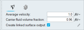
-
On the guide bar, click
to execute
the command and exit the tool.
-
Click the Outlet tool.
Figure 14. 
-
Select the face highlighted in the figure below and then click
 on the
guide bar.
on the
guide bar.
Figure 15. 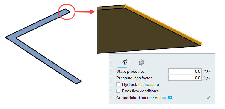
-
Click the Slip tool.
Figure 16. 
-
Select the top and bottom faces highlighted below and then click on the
guide bar.
Figure 17. 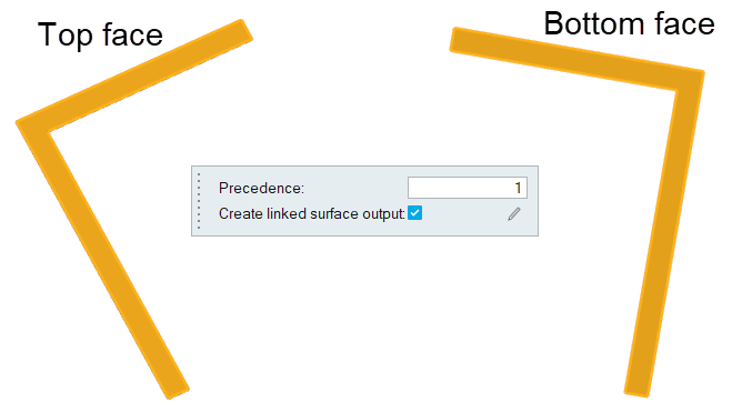
- Save the model.
Generate the Mesh
-
From the Mesh ribbon, click the
Volume tool.
Figure 18. 
-
In the Meshing Operations dialog, set the Average Element
size to 0.00104 (if not set already).
Figure 19. 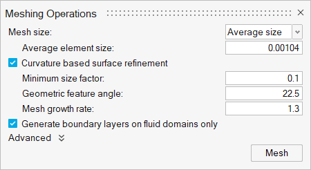
-
Click Mesh.
The Run Status dialog opens. Once the run is complete, the status is updated and you can close the dialog.Tip: Right-click the mesh job and select View log file to view a summary of the meshing process.
- Save the model.
Run AcuSolve
-
From the Solution ribbon, click the Run tool.
Figure 20. 
The Launch AcuSolve dialog opens. - Set the Parallel processing option to Intel MPI.
- Optional: Set the number of processors to 4 or 8 based on availability.
- Check the box for Use hybrid message passing and set the number of threads to the same as the number of processors.
-
Expand Default initial conditions and verify that the
Carrier field volume fraction is 1.0.
Figure 21. 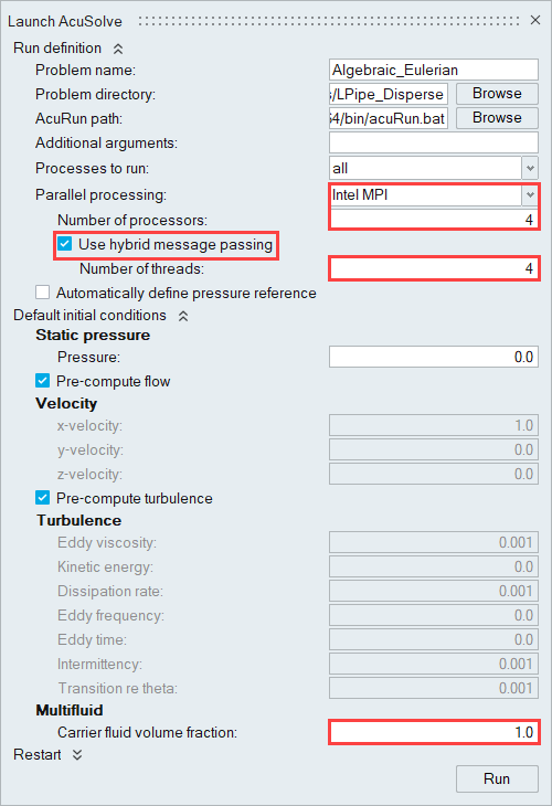
-
Click Run to launch AcuSolve.
The Run Status dialog opens. Once the run is complete, the status is updated and you can close the dialog.Tip: While AcuSolve is running, right-click the AcuSolve job in the Run Status dialog and select View Log File to monitor the solution process.
Post-Process the Results with HM-CFD Post
- Once the solution is completed, navigate to the Post ribbon.
- From the menu bar, click .
-
Select the AcuSolve
.log file in your problem
directory to load the results for post-processing.
The solid and all the surfaces are loaded in the Post Browser.
Figure 22. 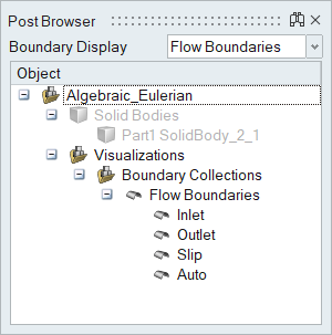
- In the Post Browser, right-click the Slip surface and select Isolate.
- Right-click Slip again and select Edit.
- In the microdialog, set the Display option to Volume fraction air.
-
Activate the Legend radio button and then click
 and set the Colormap name to
Rainbow Uniform.
and set the Colormap name to
Rainbow Uniform.
Figure 23. 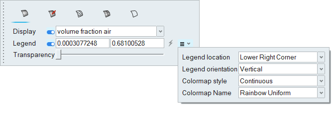
The volume fraction of air contours are displayed on the model.Figure 24. 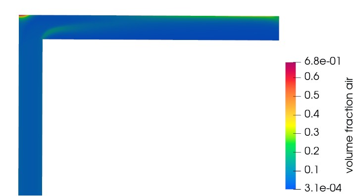
Summary
In this tutorial, you worked through a basic workflow to set up and solve a transient multiphase flow problem using the Algebraic Eulerian multiphase model in HyperMesh CFD. You started by opening the HyperMesh input file with the geometry and then defined the simulation parameters and flow boundary conditions. Upon completion of the solution by AcuSolve, you used HyperMesh CFD Post to post-process the results and create a contour plot of volume fraction.