
Signal Viewer
Use the Signal Viewer to import and treat (basic) signals in both time and frequency domains, as well as generate signals based on the most common waveforms such as step, chirp and sawtooth.
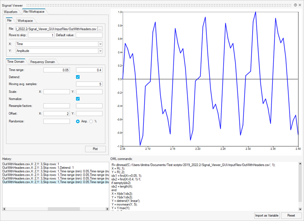
The Signal Viewer offers the following functionality:
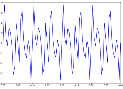
Plotting
History
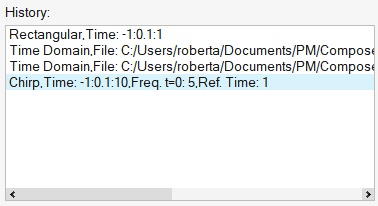
The History dialog displays the Signal Viewer events in your session. You can view or reapply any event by double-clicking it.
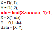
OML Command Generation
The OML Commands window autogenerates the OML syntax for producing the same output that is displayed in the Plot window. The same defined actions and visual information produced are printed in this area for reuse in an OML script.
- Run Selection: Evaluates the selected commands.
- Copy to Editor: Copies the selected commands in the active OML script editor.
If an OML script editor does not exist, or if one exists but is not active, a new OML script editor is created and the commands are pasted.
Import Data as a Variable
Use the Import as Variable button to import the visualized data as a variable. The default variable name is data. If the variable name already exists in your OML workspace, a dialog prompts you to rename or overwrite the variable. If you select Rename, a new dialog prompts you to enter a new variable name.
Reset
The Reset button clears the Signal Viewer interface and resets it to its initial state.
Waveform Tab
Create a signal based on a standard waveform, such as chirp and sawtooth.
| Waveform Option | Description |
|---|---|
| Chirp | Swept-frequency wave, in which the frequency increases or
decreases with time. If omitted, the optional parameters are:
|
| Gauss | Gaussian convolution window. If omitted, the optional parameters
are:
|
| Random | Normally distributed random signal. |
| Rectangular | Rectangular wave. If omitted, the optional parameters are:
|
| Sawtooth | Sawtooth signal. If omitted, the optional parameters are set
as:
|
| Sinusoidal | Standard sine wave. If omitted, the optional parameters are: |
| Square | Square wave. If omitted, the optional parameters are:
|
| Triangular |
|
File/Workspace Tab
Import files and select variables.
File
Import files that are supported in the dlmread command, such as delimited files.
File import options include:
- Rows to skip: The number of rows from the beginning of the file that dlmread does not read. This is useful when a file contains multiple lines of headers before the numeric data. The Signal Viewer tries to determine the number of rows to skip automatically when a file is selected.
- Default value: The value to be used in the output for empty or non-numeric values of the input file. If left empty, the value is set to 0.
If the file contains a header in its first line, the different columns will be named after this header. If not, the columns are simply called Column 1, Column 2 and so on.
If the Rows to skip or Default value values have changed, when you click the Plot button, the file is reloaded. If the file has changes since the last time it was loaded, you are prompted to select whether to reload the file or use the data already loaded in the Signal Viewer.
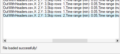
Every time the file is loaded in the Signal Viewer, an information label is shown in the lower left corner of the window.
Workspace
Select variables from the workspace. Only vectors and matrices are accepted. If the variable is a matrix, the column can also be selected.
Time Domain
Applies the following actions in the time domain:
| Time Domain Option | Description |
|---|---|
| Time Range | Cuts the signal from a lower to an upper value. |
| Detrend | Detrends the signal using the linear method, that is, removing the best fit trend. |
| Moving Avg. Samples | Applies a moving average filter based on a certain number of input samples. |
| Scale | Scales the signal in X and/or Y by a certain factor. |
| Normalize | Normalizes the signal. |
| Offset | Resamples the signal by a rational factor using a polyphase Finite Impulse Response (FIR) filter. |
| Randomize | Applies white noise in the signal either using a Signal-to-Noise
(S/N) ratio or a certain percentage of noise:
|
The actions are performed in the order that they appear, for example: Cut the signal > Detrend it > Apply moving average filter > Scale it > Normalize it > Resample it > Offset it > Randomize it
Frequency Domain
Applies the following actions in frequency domain:
| Frequency Domain Option | Description |
|---|---|
| FFT Size | Computes Fast Fourier Transform (FFT) based on the size input. If the size input is not given, the signal length is used by default. The FFT is computed, normalized and folded to generate a single-sided output. |
| Frequency Range | Applies a frequency-domain filter:
|
| Compute PSD |
|
| Window | Select the PSD checkbox to apply a windowing method to the signal
to reduce spectral leakage. If the checkbox is not selected, the PSD
is calculated without windowing. The options are:
|
| Window overlap | Number of samples that are simultaneously in different windows. To use window overlap, select the PSD checkbox and enter a windowing method other than None. If a method is not provided, the Power Spectral density is calculated without windowing. |