Inputs
Introduction
The total number of user inputs is equal to 9.
Among these inputs, 5 are standard inputs and 4 are advanced inputs.
Standard inputs
Modes of computation
There are 2 modes of computation.
The “Fast” computation mode is the default one. It corresponds to a hybrid model which is perfectly suited for the pre-design step. Indeed, all the computations in the back end are based on AC finite element computations associated to symmetrical component transformation. It evaluates the electromagnetic quantities with the best compromise between accuracy and computation time to explore the space of solutions quickly and easily.
The “Accurate” computation mode allows solving the computation with transient magnetic finite element modelling. This mode of computation is perfectly suited to the final design step because it allows getting more accurate results. It also computes additional quantities like the AC losses in winding, rotor iron losses and Joule losses in magnets.
Line-Line voltage, rms
Power supply frequency
The value of the power supply frequency of the machine: “Power supply frequency” (Power supply frequency) must be provided.
The power supply frequency is the electrical frequency applied at the terminals of the machine.
Definition mode
There are 2 common ways to define the working point. It can be defined by indicating the slip “Slip” or by defining the operating speed of the machine “Speed”.
AC losses analysi
The “AC losses analysis” (AC losses analysis required only with “Accurate” computation mode) allows to compute or not AC losses in stator winding. There are three options available:
None: AC losses are not computed. However, as the computation mode is “Accurate”, a transient computation is performed but without representing the solid conductors (wires) inside the slots. Phases are modeled with coil regions. Thanks to that, the mesh density is lower which results in a lower number of nodes and a lower computation time.
FE-One phase: AC losses are computed but only one phase is modeled with solid conductors (wires) inside the slots. The other two phases are modeled with coil regions. AC losses in winding are computed with a lower computation time than if all the phases were modeled with solid conductors. However, this can have a little impact on the accuracy of results because we have supposed that the magnetic field is not impacted by the modeling assumption.
FE-All phases: AC losses are computed, and all phases are modeled with solid conductors (wires) inside the slots. This computation method gives the best results in terms of accuracy, but with a higher computation time.
FE-Hybrid: AC losses in winding are computed without representing the wires (strands, solid conductors) inside the slots.
Since the location of each wire is accurately defined in the winding environment, sensors evaluate the evolution of the flux density close each wire. Then, a postprocessing based on analytical approaches computes the resulting current density inside the conductors and the corresponding Joule losses.
Slip
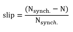
Unit can be % or PU.
Speed
When the choice of definition mode is “Speed”, the value of operating speed “Speed” (Speed) must be provided.
Advanced inputs
Number of computed electrical periods
The user input “No. computed elec. periods” (Number of computed electrical periods only required with “Accurate” computation mode) influences the accuracy of results. Indeed, the computation often leads to have transient current evolution which requiring more than an electrical period of simulation to reach the steady state over an electrical period.
The default value is equal to 2. The minimum allowed value is 0,5. The default value provides a good compromise between the accuracy of results and computation time.
Number of points per electrical period
The user input “No. points / electrical period” (Number of points per electrical period required only with “Accurate” computation mode) influences the accuracy of results (computation of the peak-peak ripple torque, iron losses, AC losses…) and the computation time.
The default value is equal to 40. The minimum recommended value is 20. The default value provides a good balance between accuracy of results and the computation time.
Skew model – No. of layers
When the rotor bars or the stator slots are skewed, the number of layers used in Flux® Skew environment to model the machine can be modified: “Skew model - No. of layers” (Number of layers for modelling the skewing in Flux® Skew environment).
Rotor initial position
The initial position of the rotor considered for computation can be set by the user in the field « Rotor initial position » (Rotor initial position).
The default value is equal to 0. The range of possible values is [-360, 360].
The rotor initial position has an impact only on the induction curve in the air gap.
Mesh order
To get the results, the original computation is performed by using a Finite Element Modeling. The geometry of the machine is automatically meshed.
Two levels of meshing can be considered for this finite element calculation: first order and second order.
This parameter influences the accuracy of results and the computation time.
By default, second order mesh is used.
Airgap mesh coefficient
The advanced user input “Airgap mesh coefficient” is a coefficient which adjusts the size of mesh elements inside the airgap. When the value of “Airgap mesh coefficient” decreases, the mesh elements get smaller, leading a higher mesh density inside the airgap, increasing the computation accuracy.
The imposed Mesh Point (size of mesh elements touching the points of the geometry), inside the Flux® software, is described as:
MeshPoint = (airgap) x (airgap mesh coefficient)
Airgap mesh coefficient is set to 1.5 by default.
The variation range of values for this parameter is [0.05; 2].
Convergence criteria on temperature
The advanced user input “Converg. Criteria on temperature” (Convergence criteria on temperature) is a percentage driving the convergence of the computation.
This advanced user input is available when the iterative thermal solving mode is selected in the thermal settings.
The iterative process (loop between electromagnetic and thermal computations) must run until the convergence criteria has been reached leading to the electromagnetic-thermal steady state. The convergence process is completed when the variation of temperature between two iterations gets lower than the ratio “Converg. Criteria on temperature” set in input.
Convergence criteria on temperature is set to 1.0 % by default.
The variation range of values for this percentage is ]0;10].
- The type of machine is Induction Machines with Squirrel cage with Inner rotor (Thermal computations are available only for inner rotor machine)
- One of the two following thermal solving modes is selected: One iteration or iterative solving mode.