Inputs

1. Introduction

The total number of inputs is equal to 16.

Among these inputs, 5 are standard inputs and 11 are advanced inputs.

The aim is to define a list of working points characterized with the torque and the speed.

To know the framework in which the working points can be selected, the torque-speed envelope is computed considering the four inputs data: the maximum line current, the maximum line-line voltage, the command mode and the maximum speed to be considered.

By default, the list of working points is built with points on the torque-speed envelope.

But, one can define a list of working points located anywhere under (or on) the torque-speed envelope.

Please refer to the section: Definition of the working point list.

2. Standard inputs

2.1 Definition of the working point list

1. Overview

   By default, the list of working points is automatically built by considering seven points on the machine torque-speed envelope. The torque-speed envelope depends on the four following input parameters:

   • Line current, rms
   • Line-Line voltage, rms
   • Command mode
   • Maximum speed

   It is also possible to define our own working point list by filling in a table with the targeted speeds and torques.

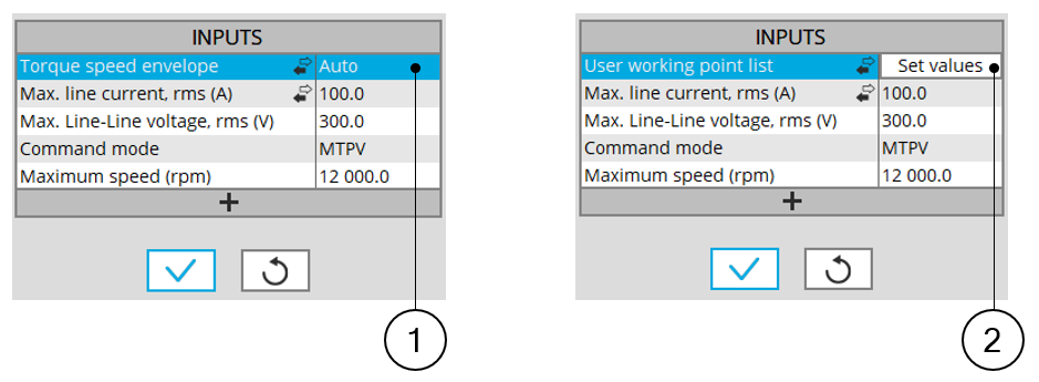
   Two ways for defining the working point list
   1	Automatic mode: working points are automatically considered on the torque-speed envelope
   2	We can define our own working point list by filling in a table with the targeted speeds and torques

2. Process to define the working point list

   Two ways are possible to define the list of working points: either filling the table line per line or by importing an Excel file in which all the working points to be considered are defined.

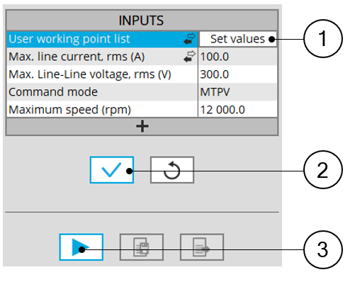
   List of working points to be defined
   1	Click on the button “Set values” of the field“ User working point list” to define the working points in a dialog box. Refer to the next illustration which shows how to fill the working point table.
   2	Button to validate the user input data
   3	Button to run the computations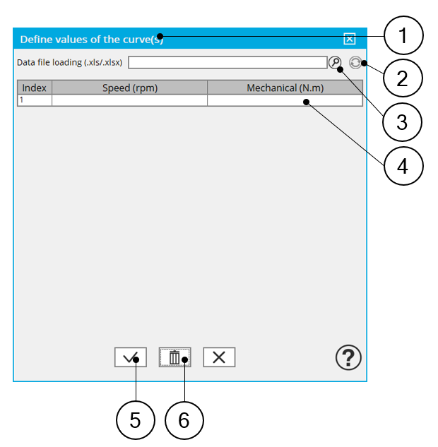

   Dialog box to define the list of working points
   1	Dialog box opened after having clicked on the button “Set values” in the field “Cycle description”
   2	Browse the folder to select an Excel file which is described the duty cycle
   3	Button to refresh the table data when the considered Excel file has been modified
   4	Fields to be filled with data to describe the duty cycle to be considered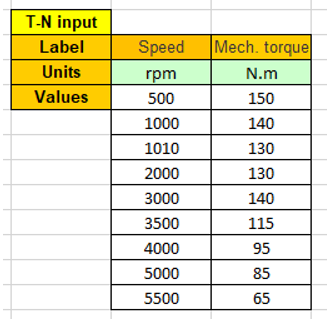

   Excel file template to define the list of working points with speed and torque data

2.2 Maximum line current, rms / Current density

There are two common ways to define the maximum line current.

Electrical current can be defined either by the current density in electric conductors or directly by indicating the value of the line current (the rms value is required).

When the choice of current definition mode is “current”, the rms value of the maximum line current supplied to the machine: “Max . l ine current, rms” ( Maximum line current, rms value ) must be provided.

When the choice of current definition mode is “density”, the rms value of the maximum current density in electric conductors “Max. Current density, rms” (Maximum current density in conductors, rms value) must be provided.

2.3 Maximum Line-Line voltage, rms

The rms value of the maximum line-line voltage supplying to the machine: “Max. Line-Line voltage, rms” ( Maximum Line-Line voltage, rms value ) must be provided.

2.4 Command mode

For any applied command mode, the process consists of computing the torque-speed envelope.

2.5 Maximum speed

The computation and analysis of the torque-speed curves are performed over a given speed range.

The maximum allowed value for the « Maximum speed » corresponds to 53000 rad/s - about 506000 rpm.

3. Advanced input

3.1 Maximum engine order / No. Points per electrical period

Two kinds of inputs are possible:

Define the Max. engine order ( Maximum engine order ) or the No. points / elec. Period ( Number of points per electric period ).

When decomposing the Maxwell pressure, applied on the stator, to get its harmonic contributions, the “ max. engine order ” ( Maximum engine order ) is required to compute its decomposition in function of the time.

At a practical point of view, when the maximum engine order is equal to N, that leads to consider 2*N computation points over a complete rotation period of the rotor.

3.2 Maximum mode / spatial order

The “ max. mode / spatial order ” ( Maximum mode / spatial order ) input allows the user to define the number of modes to be considered for the acoustic structural analysis. If the user selects 25, it means that the highest number of lobes in the stator deformation will be equal to 25 lobes. All deformations corresponding to more than 25 lobes will be dismissed.

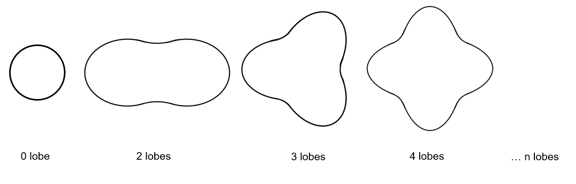Number of lobes of the stator mechanical structure

3.3 Number of computations per tooth pitch

The “ No. comp./tooth pitch ” ( Number of computations per tooth pitch ) allows to choose the number of Maxwell pressure evaluations per tooth. The more points selected, the more accurate the Maxwell pressure harmonic decomposition will be.

3.4 Number of points for speed interpolation

The “ No. points for speed interpolation ” (Number of points for speed interpolation) allows to manage the computation of the radiated sound power per engine order. It allows to manage the data interpolation between the speeds indicated as inputs. Thanks to that, the curves “Radiated sound power per engine order versus speed” and “weighted radiated sound power versus speed” can have a better discretization which leads to a better displaying of the local peaks.

The default value is equal to 100. The range of possible values is [50,300]

3.5 Number of computations for Jd,Jq

The “ No. comp. for Jd,Jq ” ( Number of computations for D-axis and Q-axis currents ) has the same definition than in the test “Performance mapping – Sine wave – Motor - Efficiency maps.

First, it is needed to compute the D-axis and Q-axis flux linkage in the J _d - J _q plane.

To get maps in the J _d - J _q plane, a grid is defined. The number of computation points along the d-axis and q-axis can be defined with the user input « No. Comp. for J _d , J _q» (Number of computations for D-axis and Q-axis currents) .

The default value is equal to 5. This default value provides a good compromise between accuracy and computation time. The minimum allowed value is 5.

3.6 Number of computations for speed

The “ No. comp. for speed ” ( Number of computations for speed ) has the same definition than in the test “Performance mapping – Sine wave – Motor - Efficiency maps.

The “ No. comp. for speed” ( Number of computations for speed ) corresponds to the number of points to be considered in the speed range from 0 to the maximum speed.

Half of these points are distributed from 0 to the base speed. The remaining points are distributed from the base speed to the maximum speed.

In both cases, base speed is considered as an additional point.

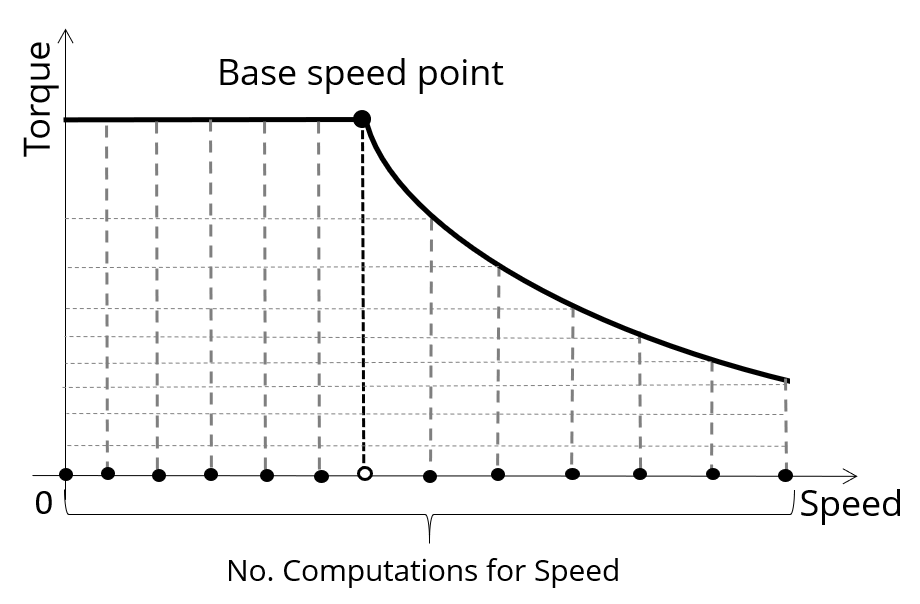Definition of the number of computations for speed

The default value is equal to 15, the minimum allowed value is 5. The maximum recommended value is 40.

3.7 Number of computations for torque

The “ No. comp. for torque ” ( Number of computations for torque ) has the same definition than in the test “Performance mapping – Sine wave – Motor - Efficiency maps.

For the speed range [N _base ; N _max. ], the number of computations for torque is imposed by the number of computations for speed in the speed range [N _base ; N _max. ] (Red points in the image shown below).

The advanced user input parameter “ No. comp. for torque ” allows to finalize the grid within the torque range [0, T (N _max. )] at the maximum speed (Black points in the image shown below).

The default value is equal to 7. The minimum allowed value is 3. The maximum recommended value is 20.

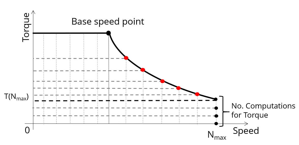Definition of the number of computations for torque – MTPV command mode

3.8 Rotor initial position mode

The “ Rotor initial position mode ” ( Rotor initial position mode ) has the same definition than in the test “Performance mapping – Sine wave – Motor - Efficiency maps.

The computation is performed by considering a relative angular position between rotor and stator.

This relative angular position corresponds to the angular distance between the direct axis of the rotor north pole and the axis of the stator phase 1 (reference phase).

According to the input “ Rotor initial position mode ”, the angular position can be defined either automatically using an internal computation process « Auto » (Automatic) or specified by the user « User » (User).

By default, the “ Rotor initial position mode ” is set to “ Auto ”.

3.9 Rotor initial position

The “ Rotor initial position ” ( Rotor initial position ) has the same definition than in the test “Performance mapping – Sine wave – Motor - Efficiency maps.

When the “ Rotor initial position mode ” is set to “ Auto ”, the initial position of the rotor is automatically defined by an internal computation process.

The resulting relative angular position corresponds to the alignment between the axis of the stator phase 1 (reference phase) and the direct axis of the rotor north pole.

When the “ Rotor initial position mode ” is set to “ User ”, the initial position of the rotor considered for computation must be set by the user in the field « Rotor initial position ». The default value is equal to 0. The range of possible values is [-360, 360].

For more detail, please refer to the section dedicated to “Rotor and stator phase relative position”.

3.10 Mesh order

To get the results, the original computation is performed using a Finite Element Modeling.

Two levels of meshing can be considered for this finite element calculation: first order and second order.

This parameter influences the accuracy of results and the computation time.

By default, second order mesh is used.

3.11 Airgap mesh coefficient

The advanced user input “ Airgap mesh coefficient ” is a coefficient which adjusts the size of mesh elements inside the airgap. When the value of “ Airgap mesh coefficient ” decreases, the mesh elements get smaller, leading to a higher mesh density inside the airgap, increasing the computation accuracy.

The imposed Mesh Point (size of mesh elements touching points of the geometry) is definined with the following parameters:

MeshPoint = (airgap) x (airgap mesh coefficient)

Airgap mesh coefficient is set to 1.5 by default.

The variation range of values for this parameter is [0.05; 2].

0.05 giving a very high mesh density and 2 giving a very coarse mesh density.