Inputs

1. Introduction

The total number of user inputs is equal to 13.

Among these inputs, 5 are default inputs and 8 are advanced inputs.

2. Standard inputs

2.1 Current definition mode

There are 2 common ways to define the electrical current.

Electrical current can be defined by the current density in electric conductors.

In this case, the current definition mode should be « Density ».

Electrical current can be defined directly by indicating the value of the line current (the RMS value is required).

In this case, the current definition mode should be « Current ».

2.2 Maximum line current, rms

When the choice of current definition mode is “ Current ”, the rms value of the maximum line current supplied to the machine: “ Max. line current, rms” ( Maximum line current, rms value ) must be provided.

2.3 Maximum current density, rms

When the choice of current definition mode is “ Density ”, the rms value of the maximum current density in electric conductors “ Max. current dens., rms” ( Maximum current density in conductors, rms value ) must be provided.

2.4 Maximum Line-Line voltage, rms

To supply the machine the rms value of the maximum Line-Line voltage: “ Max. Line-Line voltage, rms” ( Maximum Line-Line voltage, rms value ) must be provided.

2.5 Command mode

Two commands are available: Maximum Torque Per Voltage (MTPV) and Maximum Torque Per Amps (MTPA) command mode.

For the base speed point computation, both commands lead to the same results. In fact, the base speed point corresponds to the working point which maximize the mechanical torque at maximum current and at maximum voltage.

Following this, MTPA and MTPV commands give the same results on this test.

2.6 Additional losses

The “ Additional losses ” ( Additional loss percentage of electric losses ) must be provided.

It is used to consider losses which are not computed (like losses due to eddy currents, proximity effects due to electronic devices). Thus, these additional losses will be considered for computation of power balance and efficiency.

Additional losses must be evaluated as a percentage of total electrical losses (Joule + iron + additional losses).

The default value is 0. This input parameter value must be set in a range: 0% to 100% when the unit is in % and 0 to 1 when represented in “P.U.” (“Per Unit”) .

When the default value is equal to 0, it means the power balance is computed without considering additional losses.

Note: “Additional losses” input is not available in the current version (The input label is written in grey).

3. Advanced inputs

3.1 Number of computations for the control angle

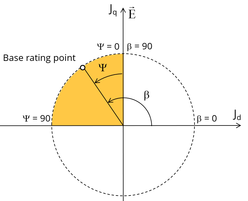
Considering the vector diagram shown below, the control angle Ψ is the angle between the electrical current (J) and the electromotive force E (Ψ = (J, E)).

The computation to get the corner point location is performed by considering control angle (Ψ) over a range of 0 to 90 electrical degrees.

The user input “ No. comp. for ctrl. angle ” ( Number of computations for the control angle) allows to choose between accuracy of results and computation time by using a number of computations between Ψ = 0º and Ψ = 90º.

The variation area for Ψ is represented by the quarter circle (colored yellow in the diagram). This discretization is necessary to find the working point corresponding to the base speed point of the torque-speed curve.

The default value of Number of computations for the control angle is equal to 5. The minimum allowed value is 5.

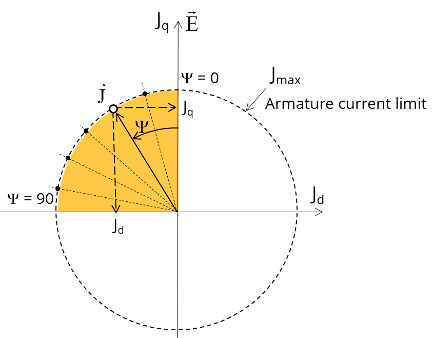Variation area for control angle Ψ

3.2 Number of computations per electrical period

For analysis like open circuit - Back-EMF or unsaturated inductances, performed over an electrical period, the user input “ No. comp. / elec. period ” (Number of computations per electrical period) influences the accuracy of results and the computation time.

Computations over electrical period are performed using a Finite Element Modelling (inside Flux software).

The default value is equal to 50. The minimum allowed value is 13. The default value provides a good compromise between the accuracy of results and computation time.

For computing the open circuit machine performance, the process is the same as in the “Characterization – Open circuit – Motor & Generator – Back-emf.

In that case, the raw computations are performed over one electrical half period. The result on a whole electrical period is rebuilt from the raw data.

The real number of computations per electrical period can be equal to the requested one +/- 1.

For the computation of unsaturated inductances, the requested number of computations over the whole electrical period is directly applied.

At last, the number of computations per electrical period displayed in outputs is always the requested one even if there is a little difference (+/- 1) with the one used for the computation of back-emf.

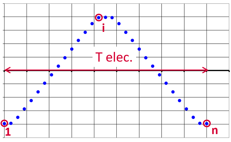Number of computations per electrical period

3.3 Number of computations per ripple torque period

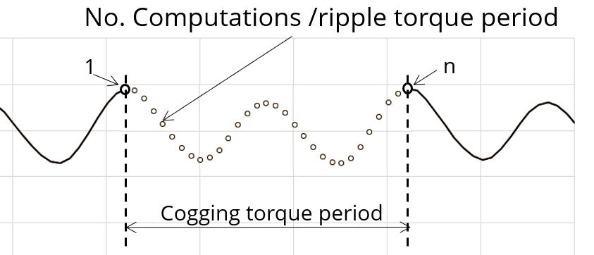
To compute peak-peak ripple torque more precisely, the user input “ No. comp. / ripple period ” (Number of computations per ripple torque period) influences the accuracy of results and the computation time.

It has also a significant impact on the computation of the magnet behavior as well as on computation of the flux density in iron.

The default value is equal to 30. The minimum allowed value is 25.

The default value provides a good compromise between the accuracy of results and computation time.

Definition of the number of computations per ripple torque period

3.4 Current coefficient

Linear conditions must be considered to compute unsaturated inductances.

To obtain a linear magnetic behavior for materials used in the magnetic circuit, the “ Current coefficient ” is used to define the corresponding maximum current which still allows linear conditions (magnetic behavior).

From practical point of view, the maximum phase current is multiplied by this current coefficient. Thus, the resulting current is used to compute the unsaturated inductances.

Note: The maximum phase current is deduced from the maximum line current defined as a user input parameter.

The range of possible values is from 0 to 1.

3.5 Rotor initial position mode

The computations are performed by considering a relative angular position between rotor and stator.

This relative angular position corresponds to the angular distance between the direct axis of the rotor north pole and the axis of the stator phase 1 (reference phase).

According to the input “ Rotor initial position mode ”, the angular position can be defined either automatically using an internal computation process « Auto » (Automatic) or specified by the user « User » (User).

By default, the “ Rotor initial position mode ” is set to “ Auto ”.

3.6 Rotor initial position

When the “ Rotor initial position mode ” is set to “ Auto ”, the initial position of the rotor is automatically defined by an internal computation process.

The resulting relative angular position corresponds to the alignment between the axis of the stator phase 1 (reference phase) and the direct axis of the rotor north pole.

When the “ Rotor initial position mode ” is set to “ User ”, the initial position of the rotor considered for computation must be set by the user in the field « Rotor initial position mode » (Rotor initial position). The default value is equal to 0. The range of possible values is [-360, 360].

For more details, please refer to the section dedicated to the rotor and stator phase relative position.

3.7 Skew model – Number of layers

When the rotor magnets or the stator slots are skewed, the number of layers used in Flux Skew environment to model the machine can be modified: “ Skew model - No. of layers” ( Number of layers for modelling the skewing in Flux Skew environment ).

3.8 Mesh order

To get the results, Finite Element Modelling computations are performed (inside Flux software).

The geometry of the machine is meshed.

Two levels of meshing can be considered: First order and second order.

This parameter influences the accuracy of results and the computation time.

By default, second order mesh is used.

3.9 Airgap mesh coefficient

The advanced user input “ Airgap mesh coefficient ” is a coefficient which adjusts the size of mesh elements inside the airgap. When the value of “ Airgap mesh coefficient ” decreases, the mesh elements get smaller, leading to a higher mesh density inside the airgap, increasing the computation accuracy.

The imposed Mesh Point (size of mesh elements touching points of the geometry), inside the Flux software, is described as:

MeshPoint = (airgap) x (airgap mesh coefficient)

Airgap mesh coefficient is set to 1.5 by default.

The variation range of values for this parameter is [0.05; 2].

0.05 giving a very high mesh density and 2 giving a very coarse mesh density.