Inputs
1. Introduction
The total number of user inputs is seven in addition to Magnet temperature entered in Settings.
Among inputs parameters, speed is the only default input parameter. Other six are available as advanced input parameters.
2.Standard inputs
2.1 Speed
Operating speed of the machine is the only standard input parameter to be used in the back-EMF test.
Note: Once the computation is performed, it is possible to change the speed and update the results instantaneously.
3. Advanced inputs
3.1 Number of computations per electrical period
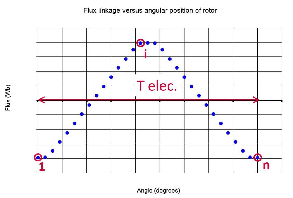
To get the Back-EMF versus time, the flux through each phase of the machine versus rotor angular position is computed.
This computation is performed using a Finite Element Modeling (Flux software).
The number of computations per electrical period “ No. comp. / elec. period ” (Number of computations per electrical period) influences the accuracy of results and the computation time.
The default value is equal to 50. The minimum allowed value is 13. This default value provides a good compromise between the accuracy of results and computation time.
The result on a whole electrical period is rebuilt from the raw data.
 |
| Number of computations per electrical period |
3.2 Maximum harmonic order
To get the Back-EMF versus time, the flux through each phase of the machine is computed versus rotor angular position.
Harmonics are extracted from the frequency analysis (F.F.T. Fast Fourier Transform) of the Back-EMF signal versus time.
The order of harmonics displayed on bar graphs and in tables can be selected with this advanced user input parameter “ Max. harmonic order ” ( Maximum harmonic order selected for visualization ).
The default value is equal to 20. The minimum allowed value is 1.
3.3 Rotor initial position mode
The computations are performed by considering a relative angular position between the rotor and the stator.
The relative angular position corresponds to the angular distance between direct axis of the rotor north pole and the axis of the stator phase 1 (reference phase).
According to the input « Rotor initial position mode » (Rotor initial position mode), the angular position can be defined either automatically using an internal process of FluxMotor « Auto » (Automatic) or specified by the user « User » (User).
By default, the “ Rotor initial position mode ” is set to “ Auto ”.
3.4 Rotor initial position
When the “ Rotor initial position mode ” is set to “ Auto ”, the initial position of the rotor is automatically defined by an internal process of FluxMotor.
The resulting relative angular position corresponds to the alignment between the axis of the stator phase 1 (reference phase) and the direct axis of the rotor north pole.
When the “ Rotor initial position mode ” is set to “ User ”, the initial position of the rotor considered for computation must be set by the user in the field « Rotor initial position ». The default value is equal to 0. The range of possible values is [-360, 360].
For more details, please refer to the section dedicated to the rotor and stator phase relative position.
3.5 Skew model – Number of layers
When the rotor magnets or the stator slots are skewed, the number of layers used in Flux Skew environment to model the machine can be modified: “ Skew model - No. of layers” ( Number of layers for modelling the skewing in Flux Skew environment ).
3.6 Mesh order
To get results, Finite Element Modelling computations are performed (Flux software).
The geometry of the machine is meshed.
Two levels of meshing can be considered: First order and second order.
This parameter influences the accuracy of results and the computation time.
The default level is second order mesh.
3.7 Airgap mesh coefficient
The advanced user input “ Airgap mesh coefficient ” is a coefficient which adjusts the size of mesh elements inside the airgap. When you decrease the value of “ Airgap mesh coefficient ”, you reduce the size of mesh elements and then increase the mesh density inside the airgap and the accuracy of results.
The imposed Mesh Point (size of mesh elements touching points of the geometry), inside the Flux software, is described as:
MeshPoint = (airgap) x (airgap mesh coefficient)
Airgap mesh coefficient is set to 1.5 by default.
The variation range of values for this parameter is [0.05; 2].
0.05 giving a very high mesh density and 2 giving a very coarse mesh density.
So, it means a need of huge numerical memory and increases the computation time considerably.