Thermal settings
1. Overview
In the thermal settings, depending of the considered test, you have two possible configurations:
- Either you can define the winding temperatures or define the physical properties of the materials needed to run the tests without any thermal computation
- Else you can choose between two other ways to run the test: iterative process until convergence or only one iteration process to perform electromagnetic computation coupled to thermal analysis.
The workflows of all these processes are described here-after.
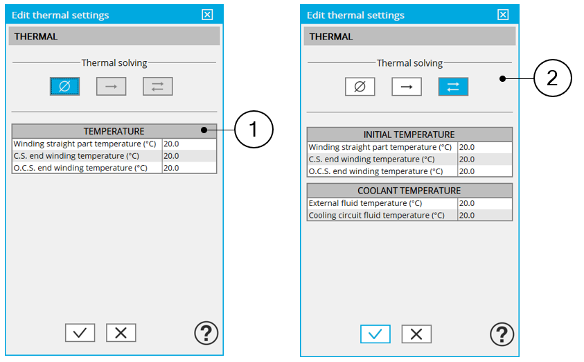 |
|
| 1 | Default mode of thermal setting for all the tests without thermal analysis |
| 2 | Thermal settings with two solving modes for all the tests with thermal analysis |
In the current version, the tests which allow using the thermal solving mode are the computations of working points defined by I, Ψ, N with motor or generator convention for Reluctance Synchronous Machines with inner rotor only.
2. Thermal settings – Without thermal solving mode
The first option of thermal setting is to run the test with only electromagnetic computation without any thermal analysis.
This option is the default for all the tests.
In this case, one must define the winding temperatures to make the corresponding material physical properties updated.
For reluctance Synchronous Machines, winding temperatures must be defined.
2.1 Temperature of winding
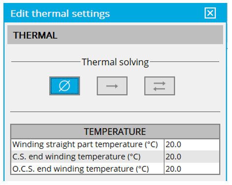 |
| Settings of winding temperature |
It is possible to define temperature of the three main parts of the stator winding:
- Winding active length temperature (part 1)
- Connection Side (C.S.) end winding temperature (part 2)
- Opposite Connection Side (O.C.S.) end winding temperature (part 3)
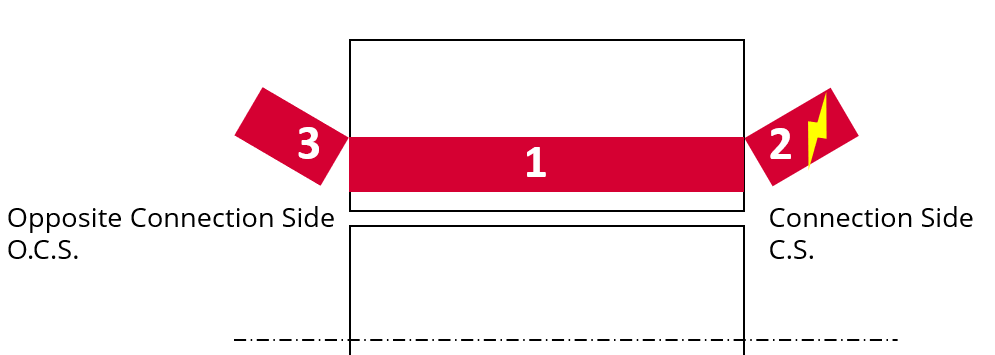 |
| Definition of the main parts of winding |
The resulting resistance of each part of the winding is updated according to the temperature:
- Winding straight part resistance (part 1)
- Connection Side (C.S.) end winding resistance (part 2)
- Opposite Connection Side (O.C.S.) end winding resistance (part 3)
The resulting resistance for the whole winding (considering the three parts described above) is computed as phase resistance and line-line resistance.
2.2 Flow chart of the tests without thermal solving mode
Below is the flow chart of computation, for test without thermal solving mode, available for all the tests.
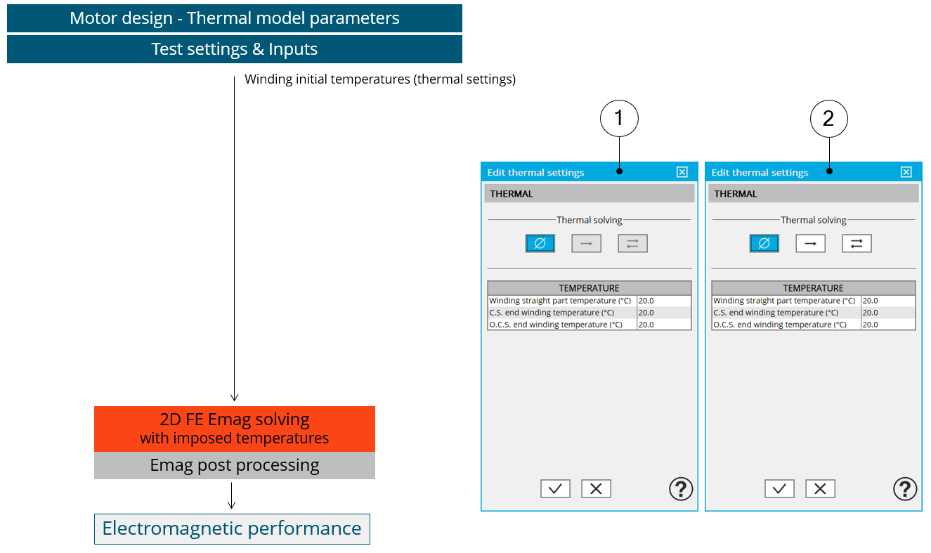 |
|
| 1 | Default mode of thermal setting for all the tests without thermal analysis |
| 2 | Thermal settings for the tests which have a thermal analysis are available |
3. Thermal settings – Thermal solving mode
3.1 Overview
The choice of thermal solving mode is available for the test dealing with the computation of working point defined by the current, control angle and speed. These solving modes involve interactions between electromagnetic and thermal computations.
Two scenarios are available: one with iterative process between electromagnetic and thermal computations until convergence, and the other with a single iteration between electromagnetic and thermal computations.
3.2 Thermal settings to initialize the test
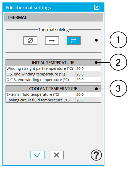
For both scenarios, here is the list of thermal settings needed to initialize the test.
 |
|
| 1 | Dialog box to define thermal setting. Iterative solving mode is selecting |
| 2 | Initial winding temperatures.These temperatures are used to initialize the electromagnetic-thermal process of computation. |
| 3 | Definition of coolant temperatures to be considered:
|
- The external fluid temperature corresponds to the temperature of the fluid surrounding the machine. It is also considered as the temperature at the “infinite” for the computation of radiation from the frame to the infinite.
- The cooling circuit fluid inlet temperature is proposed only when a cooling circuit has been added by the user in the design environment.
3.3 Flow chart of thermal solving mode – “Iterative” process
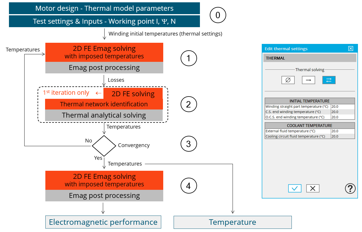
1) Flow chart or thermal solving mode test with iterative process.
 |
|
| 0 | Definition of the initial temperatures (see the list in the previous section) and working point inputs |
| 1 | 1 st electromagnetic solving (Finite Element computation) with initial temperature defined in the thermal settingsLosses are computed. |
| 2 | Based on losses and speed defined by the electromagnetic working point,The thermal characterization is performed to define the temperature distribution inside the machine.The materials physical properties corresponding to the machine active components are then updated. |
| 3 | Iterative process = loop between electromagnetic and thermal computations until the convergence on the temperature is reached (See below where can be adjusted the convergence criteria when needed) |
| 4 | A last electromagnetic solving (Finite Element computation) with final
set of temperatures is performed once the convergence on the temperature is
reached (1) . Electromagnetic performance and chart of temperatures are computed and displayed.The test outputs are illustrated in the sections dedicated to the considered tests. |
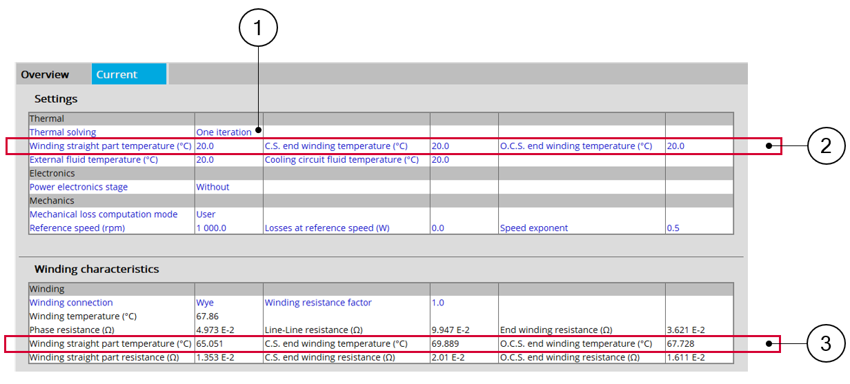
The temperatures which are considered for computing the final machine performance (step 4 in the previous flow chart) can be read in the table dealing with “Winding characteristics” of the test configuration at the beginning of result report. See below illustration.
The temperatures are also displayed in the chart of temperature and table after the electromagnetic results.
 |
|
| 1 | Initial winding temperatures |
| 2 | Resulting final temperatures which are considered for computing resulting machine performance |
2) Thermal characterization in steady state – Flow chart
This section illustrates how the thermal characterization is performed to define the temperature distribution inside the machine from a set of losses and a working point speed
This process illustrates the internal workings of the thermal characterization of the machine in the test Characterization / Thermal / Steady state
It corresponds to the second step of the previous general flow chart.
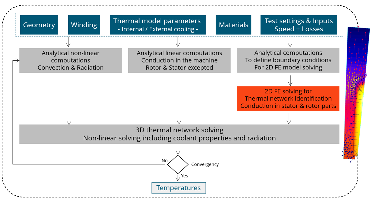 |
| Thermal test – Internal process flowchart |
The inputs of the internal process are the parameters of: Geometry, Winding, Internal cooling, External cooling, Materials, Test settings and inputs.
Then, the resulting network is extended with analytical computations to consider the 3D effect of the geometry.
The solving allows to get and to display the whole chart of temperatures of the machines.
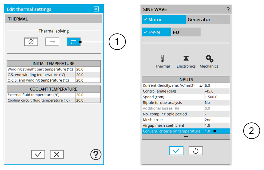
3) Iterative process – Adjustment of the convergence criteria
 |
|
| 1 | Selection of the thermal solving Iterative process in thermal settings |
| 2 | Convergence criteria can be adjusted for reaching steady state behavior.
The iterative solving is stopped once the temperature variation in the machine between two iterations is lower than the convergence criteria. A percentage close to zero gives more accurate results but takes a higher computation time. A high percentage can make the convergence shorter but decreases the accuracy of the results. |
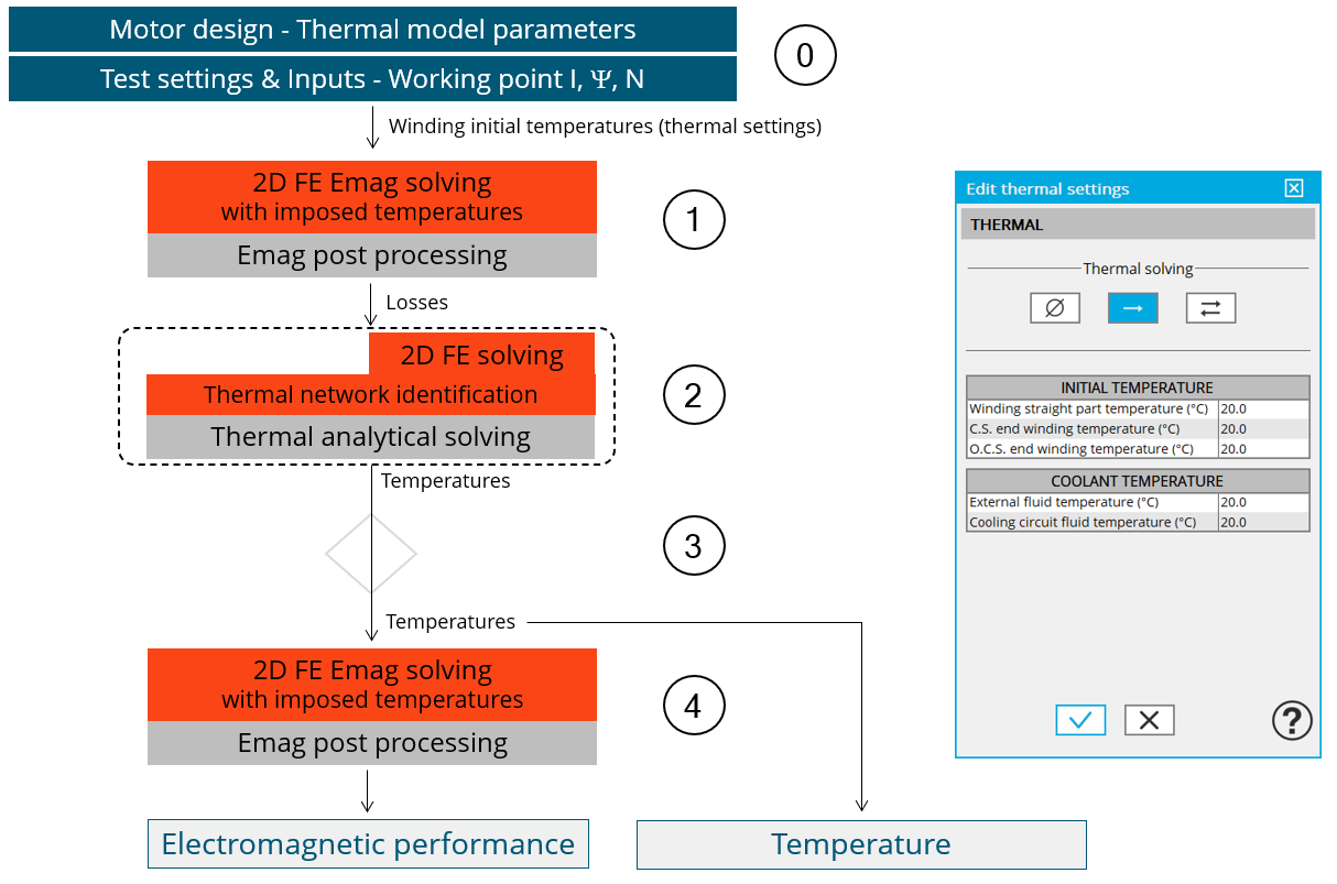
3.4 Flow chart of thermal solving mode – “One iteration” process
1) Flow chart of the thermal solving mode test with a single iteration.
 |
|
| 0 | Definition of the initial temperatures (see the list in the previous section) and working point inputs |
| 1 | 1 st electromagnetic solving (Finite Element computation) with initial temperature defined in the thermal settingsLosses are computed. |
| 2 | Based on losses and speed defined by the electromagnetic working point,The thermal characterization is performed to define the temperature distribution inside the machine (1) .The materials physical properties corresponding to the machine active components are then updated. |
| 3 | There is not an iterative process = only one iteration is carried out. |
| 4 | A last electromagnetic solving (Finite Element computation) with final set of temperatures got after convergence is performed (2) .Electromagnetic performance and chart of temperatures are computed and displayed.The test outputs are illustrated in the sections dedicated to the considered tests. |
- It corresponds to what is performed to make the thermal characterization of the machine in the test Characterization / Thermal / Steady state
- The temperatures which are considered for computing the final machine performance (step 4 in the previous flow chart) can be read in the table dealing with “Winding characteristics” of the test configuration at the beginning of result report. See below illustration.
The temperatures are also displayed in the chart of temperature and table after the electromagnetic results.
 |
|
| 1 | Initial winding temperatures |
| 2 | Resulting final temperatures which are considered for computing resulting machine performance |