チュートリアルレベル:アドバンストLearn how to set up a model of a controlled system, prepare it for interaction with HyperStudy, and perform an optimization in AltairHyperStudy.
重要:Available only with Twin Activate commercial edition.
このチュートリアルのファイル
PID.scm、PID Optimization.hstx
チュートリアルで構築するモデルの完成版と、チュートリアルを完了するために必要なすべてのファイルは、デモブラウザ:Tutorial Models > Integration and Collaboration > Optimizing a Controller with から入手できます。HyperStudyまたは、以下の場所から入手できます:<installation_directory>/Tutorial
Models/Integration and Collaboration/Optimizing a Controller with HyperStudy
Overview
This overview discusses the objective, system description, performance metric, model
components, key observations, steps, expected output, and challenges of the Optimizing a
Controller with HyperStudy tutorial.
Objective
The goal of this problem is to optimize the tuning of a
Proportional-integral-derivative (PID) controller
(Kp,
Ki,
Kd) for a second-order
system to minimize the Integral of Time-weighted Absolute Error (ITAE). The ITAE is
a widely used performance metric that evaluates the control system's response. It
emphasizes early error correction and penalizes errors over time.
Adjustment (optimization) of the three parameters can be a complex task that requires
automation and mathematical optimization. This tutorial demonstrates how to couple
Twin Activate and HyperStudy
to perform parameter optimization.
System Description
The system being controlled is a second-order plant represented by the transfer
function:
This transfer function models a generic second-order system with a damping ratio (ζ =
0.5) and natural frequency (ωn = 1).
A PID controller is used to control the plant and minimize the error between the
reference input (step signal) and the plant output. The controller has three tuning
parameters:
Kp = Proportional gain
Ki = Integral gain
Kd = Derivative gain
These parameters influence the system's rise time, overshoot, settling time,
and steady-state error.
A step input is used as the reference signal. The step input starts at 0 and
transitions to a value of 1 at t = 0. The system's task is to
track this step input.
Performance Metric: ITAE
The ITAE (Integral of Time-weighted Absolute Error) is used as the performance
metric. It is defined as:
Where:
e(t) is the error between the reference
input and the plant output ().
t is time, which weights the error more heavily as time
progresses.
T is the total simulation time.
The goal is to minimize ITAE, which means:
Reduce large errors early in the response (where t is
small).
Prevent sustained errors later in the response (where t is
large and errors are penalized more).
Model Components
PID Controller:
Inputs: Error signal (e(t)).
Outputs: Control signal to the plant.
Role: Adjust the plant's output to minimize the error and stabilize the
system.
Second-Order Plant:
Inputs: Control signal from the PID controller.
Outputs: System response
(y(t)).
Role: Represents the dynamics of the system being controlled.
Summation Block:
Inputs: Reference signal (r(t))
and plant output (y(t)).
Outputs: Error signal ()
Role: Computes the error, which is used by the PID controller.
Step Input:
Initial value: 0.
Final value: 1.
Role: Provides the reference signal for the system to track.
ITAE Calculation:
Computes : The absolute value of the error.
Multiplies by time (t): Penalizes errors over
time.
Integrates over time (T): Accumulates the weighted
error.
Key Observations
Importance of Proper Gains:
Kp: Affects the
system's responsiveness.
Ki: Eliminates
steady-state error.
Kd: Reduces overshoot
and oscillations. Improper gains can lead to instability, overshoot, or
sluggish behavior.
Why ITAE is Used:
ITAE prioritizes correcting early errors.
Penalizes systems that take a long time to settle or exhibit sustained
oscillations.
Simulation Time: The simulation must run long enough (T=10
to 30 seconds) to capture the system's transient and steady-state behavior.
Steps in the Model Setup
Define the Plant: Use a transfer function block to model:
Add the PID Controller: Use a PID block to process the error signal and generate
a control signal.
Compute Error (e(t)): Use a summation
block to compute
Reference Signal: Use a step input block with:
Initial value: 0
Final value: 1
Step time: 0
Calculate ITAE: Use blocks to:
Compute the absolute error ().
Multiply by the time signal (t).
Integrate the result to obtain ITAE.
Display Results: Use scopes to display:
The system response (y(t))
The accumulated ITAE value
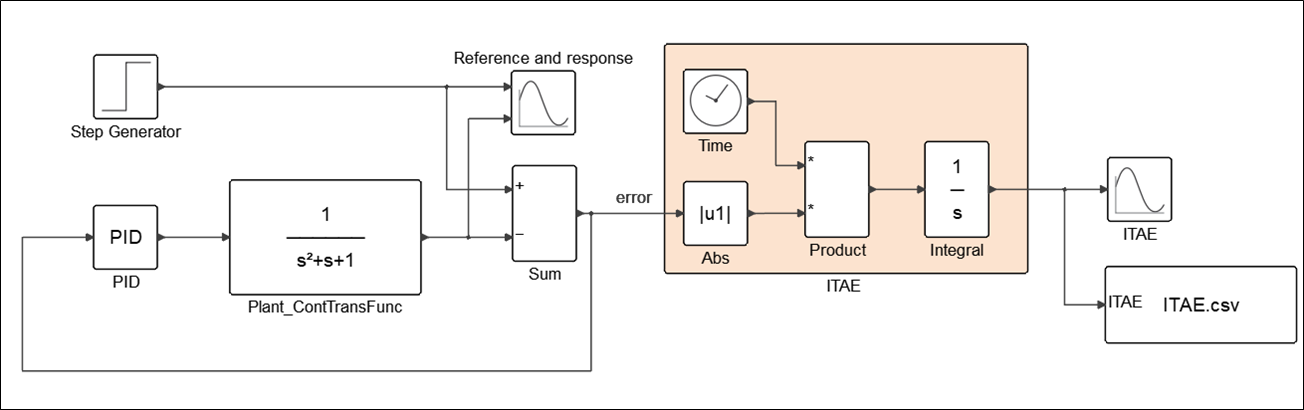
図 1. The PID Model with ITAE
Expected Output
System Response: The plant output (y(t))
should track the step input (r(t)) with
minimal overshoot, fast rise time, and minimal steady-state error.
Properly adjust Kp,
Ki, and
Kd to balance
responsiveness and stability.
Avoid overshoot, instability, or sluggish response.
ITAE Calculation: Ensure accurate computation of the absolute error and its
time-weighted integral.
System Dynamics:
Understand how the second-order plant interacts with the PID
controller.
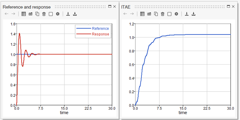
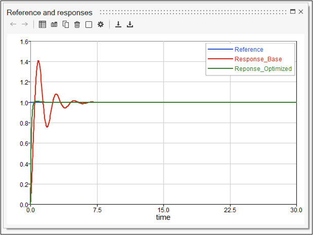
The figure below shows the reference and response signals, along with
the nature of ITAE of this model for the base model.
図 2. Reference and Response Signals and ITAE Before Optimization
Prepare the Model in Twin Activate for Optimization
Prepare the model by adding values to the initialization script and adding a ToCSV
block.
When the model is ready and running well, make the following changes.
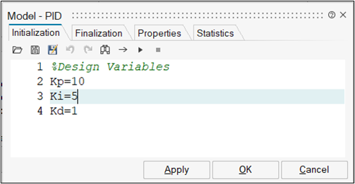
Add the following values of
Kp,
Ki,
Kd to the initialization
script:
Kp=10
Ki=5
Kd=1
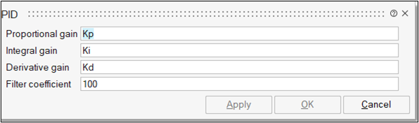
図 3. Initialization Script Where Design Variables are Declared Use these variables in the PID block.図 4. Variables Used to Define the Gains in the PID Block
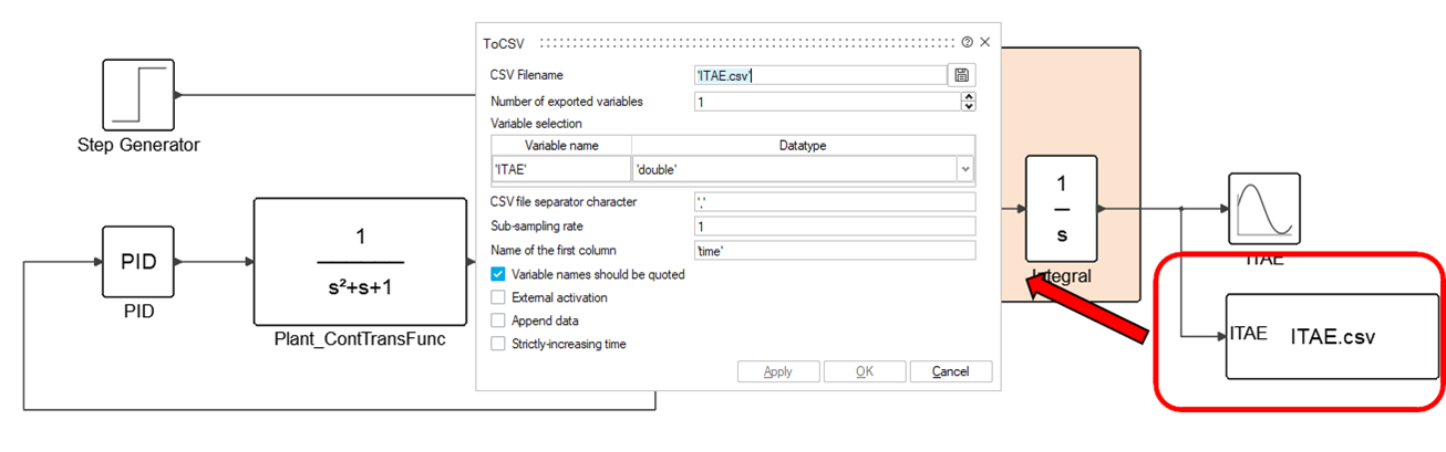
Add a ToCSV block with the following values:
CSV Filename: 'ITAE.csv'
Number of exported variables: 1
Variable name: 'ITAE', Datatype:
'double'
Sub-sampling rate: 1
Name of the first column: 'time'
Select Variable names should be quoted
When HyperStudy calls Twin Activate during any run, it expects that a CSV file is
created. This CSV file is used as an output source. It should contain all the
response vectors that are required in HyperStudy.
In this case, you need to dump the ITAE values, into a CSV file. The final
value of this vector is used in HyperStudy to define
a response.図 5. The PID model with ITAE
The model is now ready to be linked with HyperStudy.
Optimize using HyperStudy
These steps show you how to perform an optimization in HyperStudy.
HyperStudy is a multi-disciplinary design exploration,
study, and optimization software. HyperStudy lets you
explore, understand, and improve your system's designs using methods such as
design-of-experiments and optimization. HyperStudy
generates intelligent variations of the parameters of any system model and reveals
relationships between these parameters and the system responses.
HyperStudy provides engineers and designers a
user-friendly environment to:
Improve Design Performance and Quality: It includes state-of-the-art,
innovative optimization, design of experiments, and stochastic methods for
rapid assessment and improvement of design performance and quality.
Reduce Development Time and Costs: It helps engineers reduce trial-and-error
iterations and hence helps to reduce both the design development and testing
time.
Increase Productivity through Easy-to-use Environment: HyperStudy's step-by-step process guides you in
setting up and carrying out design studies. Its open architecture allows
easy integration with 3rd party solvers.
Perform Powerful Dataset Analysis: A comprehensive set of post processing
and data mining methods simplify and aid an engineer’s job of analyzing and
understanding large simulation datasets.
Improve Simulation Correlation: HyperStudy's
optimization capabilities can be applied to improve correlation of analysis
models with test results or with other models.
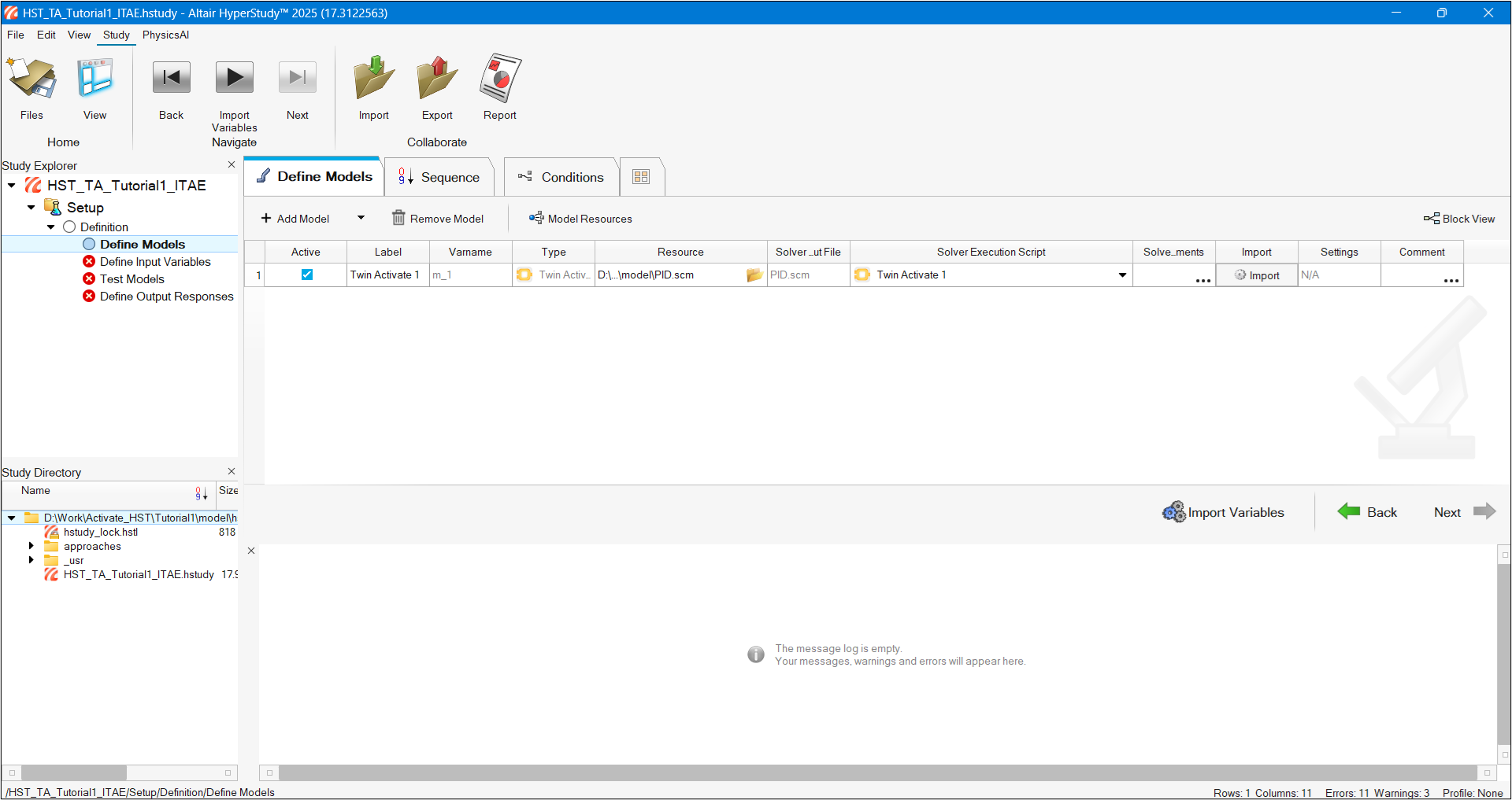
Add the SCM file prepared earlier. For
Type, choose Twin Activate.
Set Solver execution script is set to Twin Activate and ensure the path to the script is defined
correctly.
The path can be defined in Edit > Register Solver Script.図 6. Twin Activate Model Added in HyperStudy
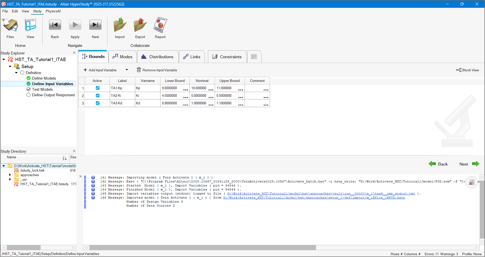
Click Import or Import Variables
to import all the design variables defined in the initialization script of the
Twin Activate file.
注: All independent variables are imported as design
variables in HyperStudy. The Define Input
Variables tab looks like the image below.
図 7. Design Variables in HyperStudy
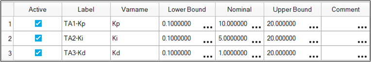
Change the lower and upper bounds to 0.1 and
20, respectively, for all three design
variables.
図 8. Upper and Lower Bounds
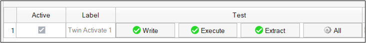
In the Test Models tab, click Run Definition.
If the model runs without errors, three green check marks are shown under
Test.
図 9. Indication that the Model has Run Successfully
The stdout.txt file listed in the message log should not
show any errors. This means that the model has successfully run from HyperStudy.
Click Define Output Responses.
Click Data Sources.
You should see that two output data sources have been added: ToCSV_time and
ToCSV_ITAE. These represent the two columns of data from the
ITAE.csv file. You only need the last value of the
ToCSV_ITAE vector.
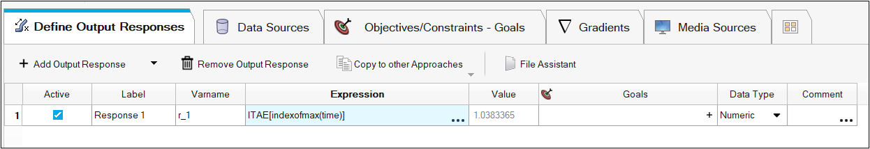
Click Define Output Responses, and then click
Add Output Response.
Under expression type, enter ITAE[indexofmax(time)], and
then click Evaluate.
The last value is now shown in the Value column.図 10. Using the Last Value of ITAE as a Response The model setup in HyperStudy is now complete.
To add an optimization study, right-click in the left browser window or click Next > Add in the Define Output Responses tab.
For Definition from, select Setup as
the value.
The model, design variables, and output responses are created in the new
optimization study.
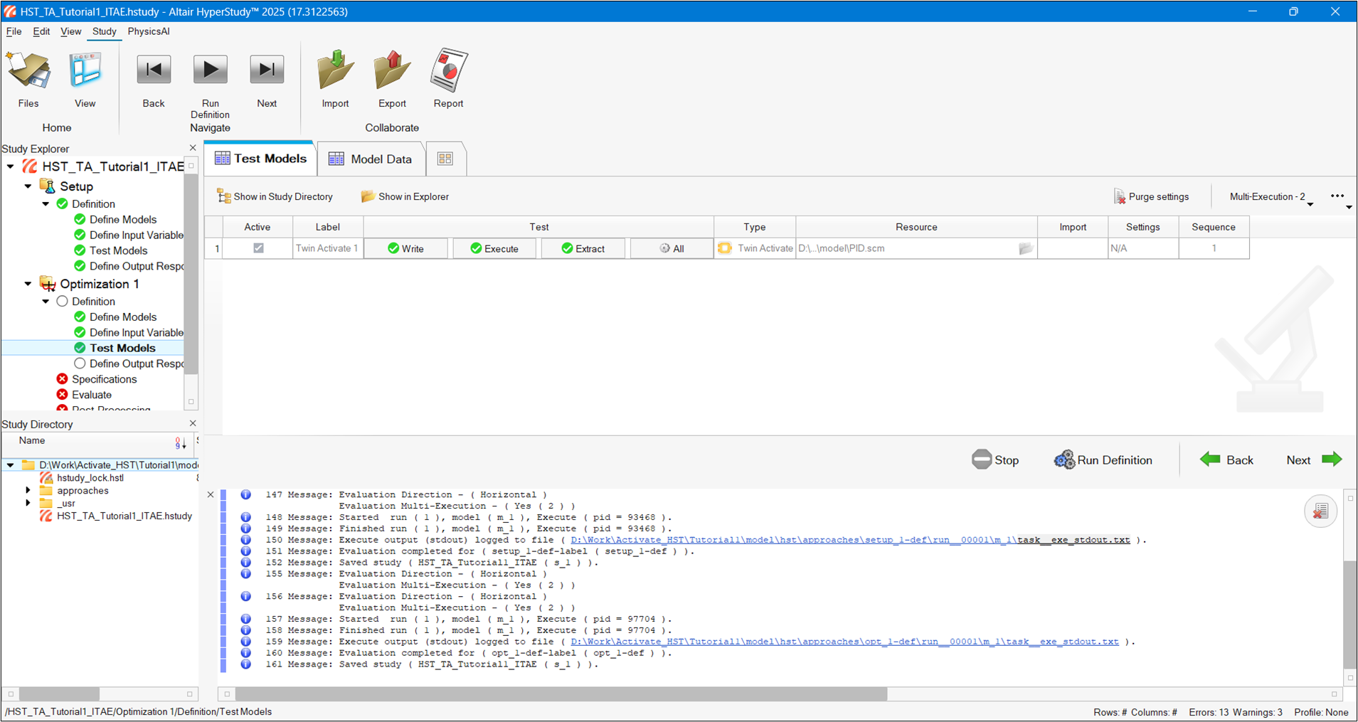
From the Test Models tab in the browser, click
Run Definition.
Ensure the model runs without any errors.
図 11. Running the Model in the Optimization Study
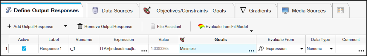
From the Define Output Responses tab in the browser on
the left, select Minimize > Goals.
The optimization algorithm tries to minimize the value of last value of
ITAE.
注: You might have to click
Evaluate to populate the value of the
response.
図 12. Defining the Goal in HyperStudy
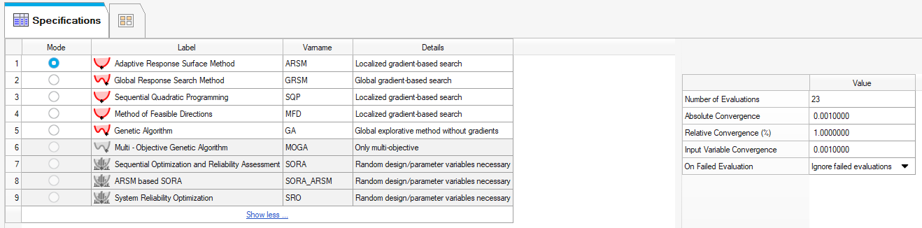
Click Specifications in the browser.
Select the Adaptive Response Surface Method as the
optimization mode on the left side of the tab. Set the following parameters on
the right side:
Number of Evaluations: 23
Absolute Convergence: 0.001
Relative Convergence (%): 1.000
Input Variable Convergence: 0.001
On Failed Evaluation: Ignore failed evaluations
Click Apply to use the modified settings.
図 13. Optimizer Settings
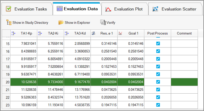
Open the Evaluate tab in the browser, and then click
Evaluate Tasks.
When the optimization is complete, look for the row highlighted in
green. This lists the optimized value of ITAE and the corresponding design
variable values (Initial: 1.038; Optimized: 0.0402).
図 14. Optimum Values of Design Variables
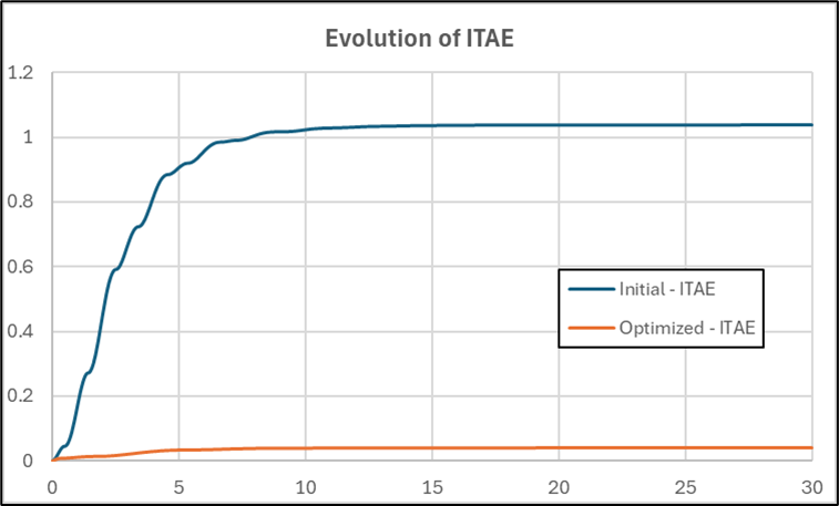
The CSV files from run folder 20 (optimized solution) can be compared
with the initial value in run folder 1.
図 15. Reduction of ITAE using Optimized Values of the Design
Variables
図 16. Comparison of Response from Base Values of PID and Optimized
Values of PID
As can be seen in the above figure, the response from the optimized
values of Kp,
Ki,
Kd happen to produce a
much smoother and better response.