
Redundant Constraints
Learn how redundant constraints appear in your model and how they could impact your solution.
What are redundant constraints?
Redundant constraints occur in rigid multi-body dynamics when multiple rigid joints or certain types of inputs each attempt to control one or more of the same degrees of freedom (DOF) of part.
A flexible (finite element) body can have hundreds or thousands of DOF, due to the many nodes that connect mesh elements together. Adding a joint to a flexible part constrains the nodes near the point of the constraint, but the remaining nodes across the rest of the part are free to move so the part can flex. Your can add additional joints without overconstraining the part.
A rigid body only has six DOF. The entire body can only move in space along three translational DOF (x, y, z) and rotate about three DOF (x, y, z). Adding a single kinematic joint to a rigid part constrains one or more of the part’s six DOF. Therefore, for rigid parts, adding more than one kinematic joint of certain types to a single part can quickly result in overconstraining it.
Rigid (kinematic) joints are idealized joints that remove DOF based on their type. They cannot deform like real-world joints. Here are some examples of rigid joints and the DOF they remove:
| Joint Type | Removes DOF | Allows |
|---|---|---|
| Hinge or Pin | 5 | 1 Rotation |
| Cylindrical or Sliding Pin | 4 | 1 Rotation 1 Translation |
| Ball and Socket | 3 | 3 Rotations |
| Translational | 5 | 1 Translation |
| Planar | 3 | 1 Rotation 2 Translations |
Additionally, non-force-based motors and actuators that do not use a controller are considered constraints. They remove DOF in the direction of their motion.
For determining the total system DOF of the model, a formula called a Gruebler count is used:
Moving Parts DOF - Constrained DOF = Total System DOF
How Are Redundant Constraints Constructed?
Consider the scenario below:
- A (rigid) door hanging on two (rigid) hinges, which in turn are connected to the door frame, which is grounded using kinematic joints.
- Gravity is the only load on the door.
When building a multi-body model, there is a natural tendency to want to connect the door to the frame using as many hinges as there are in the real world. However, this can lead to redundant constraints.
What Made the System Redundant?
In the scenario above, when the first hinge joint was added to connect the door to ground, it removed five of the door’s six available DOF. The solution was fully defined with 1 rotational DOF, rotation about the hinge axis. When the second hinge joint was added, it attempted to remove the same five DOF the first joint removed. In the end, the two joints became redundant with one another. The constraint equations introduced by the second joint were identical to the first and not necessary for the solution.
Below is an example of a completed Gruebler Count for the scenario above.
| Part | DOF |
|---|---|
| Door | +6 |
| Hinge 1 | -5 |
| Hinge 2 | -5 |
| Total | -4 |
Consequences of Redundant Constraints
At the time of solve, if redundant constraints are present, the solver will attempt to remove the redundancies by automatically removing the responsible constraint equations. This is a semi-random process by the solver. As a result, there will be no reaction force or moment results on any of the constraint DOF that were removed. For example, a hinge joint allows one for rotational DOF. If any of its constrained translational DOF are removed by the solver, there will be no linear reaction force results for x, y, or z for the joint.
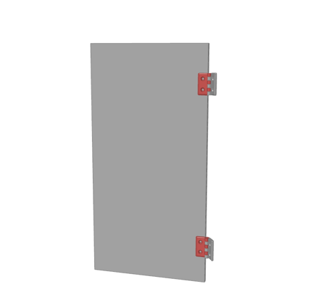
Example 1: Door On Two Hinges
In the image below, the door on the left is modeled differently from the door on the right. Notice the difference in the types of force reactions and their directions.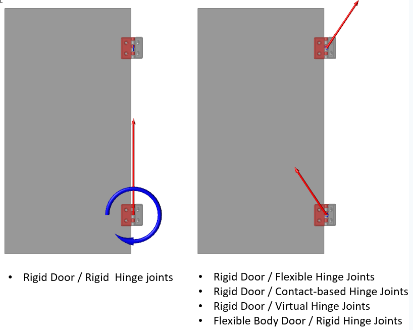
The door on the left has a single reaction force and bending moment on only one of the hinges instead of both. This is because the solver determined the upper hinge constraints were redundant with the bottom, so it removed the associated constraint equations. As a result, no reaction forces were calculated for the constraints that were removed. On the other hand, using other connections methods, the results for the door on the right match empirical solutions and show the proper reaction types and directions.
Example 2: Shaft Supported by Bearings
In the image below, the shaft is supported by two bearings (rigid hinge joints). When building a multi-body model, there is a natural tendency to want to connect the shaft to the bearings using as many bearings as there are in the real world. This can lead to redundant constraints.
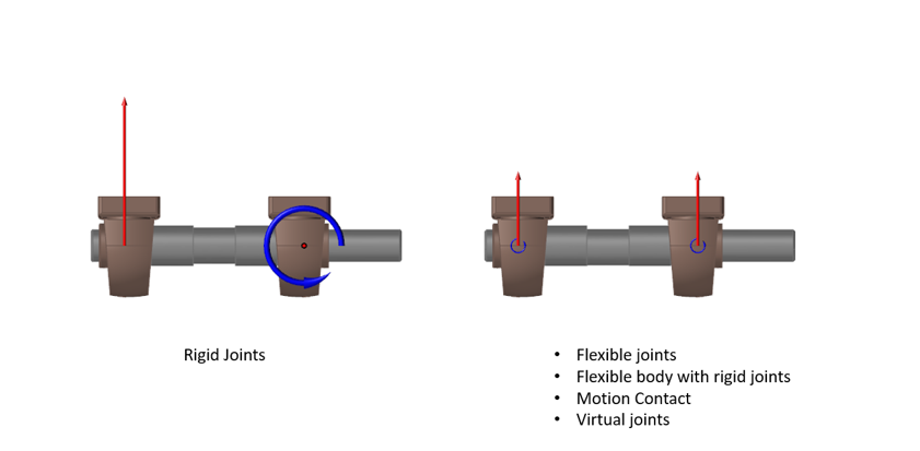
The shaft on the left has a single reaction force and bending moment, whereas it should have two equal vertical reactions, as seen in the image on the right. Two rigid hinge joints are not needed for the virtual representation of this rigid body problem. The solver determined one or more of the hinge constraints were redundant with the other and chose to remove the conflicting constraint DOF. As a result, no reaction forces were calculated for the removed constraints. The results for the shaft on the right are correct.
How to Avoid Creating Redundant Constraints:
- Use Flexible joints. Inspire Motion employs Flexible joints by default to prevent redundant constraints when modeling with rigid parts. Flexible joints use a balance of forces instead of constraint equations, which does not result in redundant constraints. Several flexible joints can be added to a rigid part and not result in redundant constraints.
- Use Flexible bodies, which are made up of hundreds or thousands of DOF. Multiple rigid kinematic joints can be added to a flexible part without overconstraining it. This is also a good option when modeling joint friction, as joints must be rigid to account for friction.
- Use Motion Contact. If the geometry allows, motion contact can be used in place of joints. Contacts do not utilize constraint equations and therefore cannot introduce redundancies.
-
Use Virtual joints. A virtual joint will provide the same constraint behavior as an ideal kinematic joint, with the exception that, due to its method of solution, it cannot introduce redundancies. Virtual joints employ another numerical approach to solving the general equations of motion.
Final Note:
Redundant constraints are typically only of concern when forces or moments are being sought. Not all overconstrained models will produce incorrect results. It depends on where results are being sought and which types. For example, the shaft may have certain redundancies that prevent the proper vertical reaction forces from being produced, but the angular velocity will be correct. The Force Explorer is a good tool for quickly validating the presence of certain load reactions at the various joints.