OS-V: 1110 Vibrating Sphere: Exterior Acoustic Analysis using Infinite Elements (IE) and Adaptive Perfectly Matched Layer (APML) Methods
Acoustic modeling in finite and semi-infinite domains is essential in the prediction of quantities such as external and radiated noise in vibro-acoustic problems.
APML is a popular way of modeling these domains. If sound pressure at microphone locations is to be calculated because of sound propagating through sections of the fluid domain and through panels, this method shows the fidelity of various vibrating sound sources, such as speakers, as it allows prediction of radiated noise.
Model Files
Benchmark Model
The sphere is of 1 m radius.
All the nodes of the model are constrained to six degrees of freedom (123456), along with an enforced velocity of a 1.0 m/s amplitude on SPCD via RLOAD1 in DOF 3.
The loading frequencies at which the responses are calculated are specified using the FREQ1 entry starting from 50 Hz to 160 Hz in increments of 10 Hz.
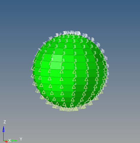
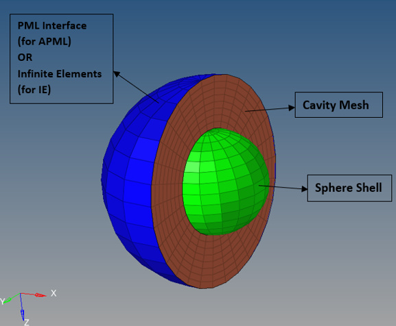
For APML, the entire vibrating structure is enclosed with an acoustic cavity mesh and further adding a layer of PML elements on this enclosed acoustic cavity mesh. A minimum of one layer of fluid elements will be defined on the surface of the structural domain of interest. Then, the APML elements, CACPML3 and CACPML4 will only be defined on the topmost surface of the fluid elements (Figure 2).
Similarly for IE, the vibrating structure is enclosed with an acoustic cavity mesh and a layer of Infinite Elements (CACINF3 and CACINF4) on the enclosed acoustic cavity mesh is added.
Units: m, s, Pa, kg/m3
Material
Sphere shell is aluminum which is specified using MAT1 Bulk Data Entry. Fluid material properties (bulk modulus, speed of sound, fluid density) are specified for the fluid cavity elements on the MAT10 Bulk Data Entry. For this model, the fluid is assumed to be air.
Sound pressure can be measured on the receiver grid points (microphone locations). These microphones are located at coordinates z = -4 m and z = 10 m as fluid grids 9003 and 9000, respectively in the frequency range 50 to 160 Hz.
The spatially dependent amplitudes of the field quantities are identified as:
Sound pressure is defined as:
- Density of medium
- Speed of sound in the medium
- Wave number (=circular loading frequency/speed of sound)
- Radius of the sphere
- Prescribed oscillatory velocity
- Radial distance of the microphone location
- Polar angle of microphone location (angle measured about the +ve z axis)
Results
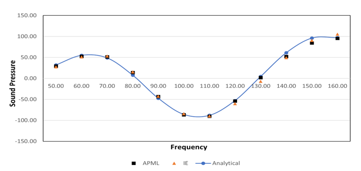
Sound Pressure versus Frequency for two microphone locations is plotted.
Adaptive Perfectly Matched Layer (APML), Infinite Elements (IE) and Analytical results are compared.
| APML | IE | |
|---|---|---|
| Z = 10 | 8.55% | 24.46% |
| Z = -4 | 7.79% | 11.15% |
- Microphone Pressure versus Frequency at z = 10 m
Figure 3. Real 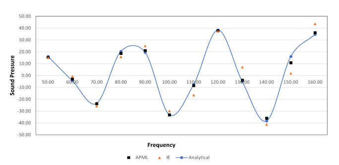
Figure 4. Imaginary 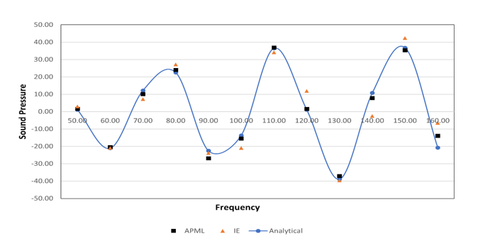
- Microphone Pressure versus Frequency at z = 10 m
Figure 5. Real 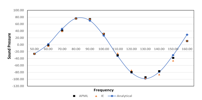
Figure 6. Imaginary