OS-V: 1200 Pulsating Sphere: Exterior Acoustic Analysis using Infinite Elements (IE) and Adaptive Perfectly Matched Layer (APML) Methods

Acoustic modeling in finite and semi-infinite domains is essential in the prediction of quantities such as external and radiated noise in vibro-acoustic problems.

APML is a popular way of modeling these domains. If sound pressure at microphone locations is to be calculated because of sound propagating through sections of the fluid domain and through panels, this method shows the fidelity of various vibrating sound sources, such as speakers, as it allows prediction of radiated noise.

Model Files

Before you begin, copy the file(s) used in this problem to your working directory.

Benchmark Model

The sphere is of 1 m radius.

All the nodes of the model are constrained to six degrees of freedom (123456), along with an enforced velocity of 1.0 m/s amplitude on SPCD via RLOAD1 in DOF 3 (in radial direction) in the spherical coordinate system.

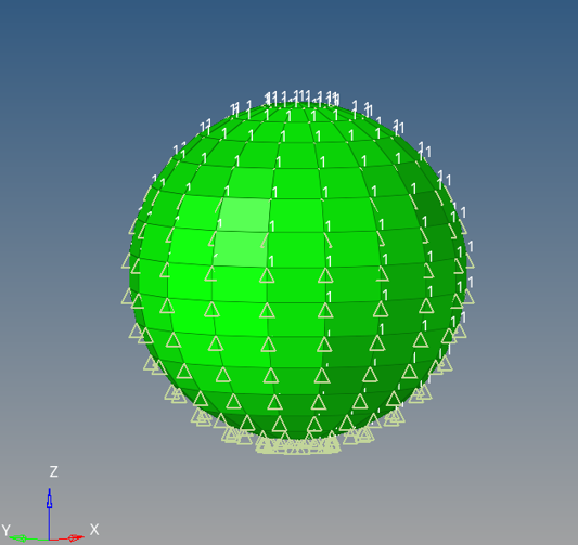
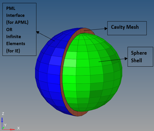
For APML, the entire vibrating structure is enclosed with an acoustic cavity mesh and further adding a layer of PML elements on this enclosed acoustic cavity mesh. A minimum of one layer of fluid elements must be defined on the surface of the structural domain of interest. Then, the APML elements, CACPML3 and CACPML4 will only be defined on the topmost surface of the fluid elements (Figure 2).

Similarly for IE, the vibrating structure is enclosed with an acoustic cavity mesh and a layer of Infinite Elements (CACINF3 and CACINF4) on the enclosed acoustic cavity mesh is added.

Units: m, s, Pa, kg/m³

Material

Sphere shell is aluminum which is specified using MAT1 Bulk Data Entry. Fluid material properties (bulk modulus, speed of sound, fluid density) are specified for the fluid cavity elements on the MAT10 Bulk Data Entry. For this model, the fluid is assumed to be air.

The loading frequency input is specified using FREQi card with frequencies 54.59 Hz, 109.18 Hz and 163.77 Hz. The sphere is vibrating in air with unit radial velocity at integer wave numbers $k$ = 1, 2, 3.

Microphones, where the sound pressure is measured, are located at 2 m, 4 m, 10 m, 50 m and 100 m.

Analytical Calculation

(1)

p = \frac{- i k a^{2} {\hat{v}}_{S}}{r (1 - i k a)} e^{i k (r - a)} ρ c

Where,

$ρ$: Density of medium
$c$: Speed of sound in the medium
$k$: Wave number (=circular loading frequency/speed of sound)
$a$: Radius of the sphere
${\hat{v}}_{C}$: Prescribed structural radial velocity on surface of the sphere
$r$: Radial distance of the microphone location

Results

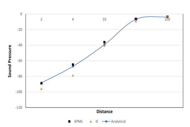
Sound Pressure versus Microphone location for three frequencies corresponding to wave numbers $k$ of 1, 2 and 3 are plotted.

Adaptive Perfectly Matched Layer (APML), Infinite Elements (IE) and Analytical results are compared.

The goal of this project is to understand how OptiStruct methods APML and IE correlate with the analytical method and to check the accuracy of the OptiStruct results with the Analytical results.

Table 1. Average Percentage Difference of Sound Pressure between APML and IE with Analytical
	APML	IE
$k$ =1	10.59%	9.42%
$k$ =2	6.30%	24.2%
$k$ =3	6.12%	12.05%

From the plots below, APML and IE correlate with the analytical method.

Microphone Sound Pressure versus Distance ( $k$ = 1)
Figure 3. Real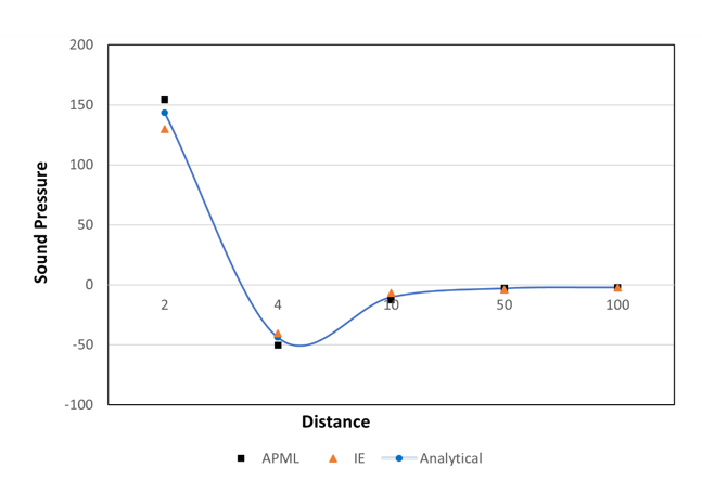

Figure 4. Imaginary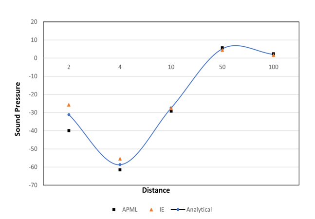
Microphone Sound Pressure versus Distance ( $k$ = 2)
Figure 5. Real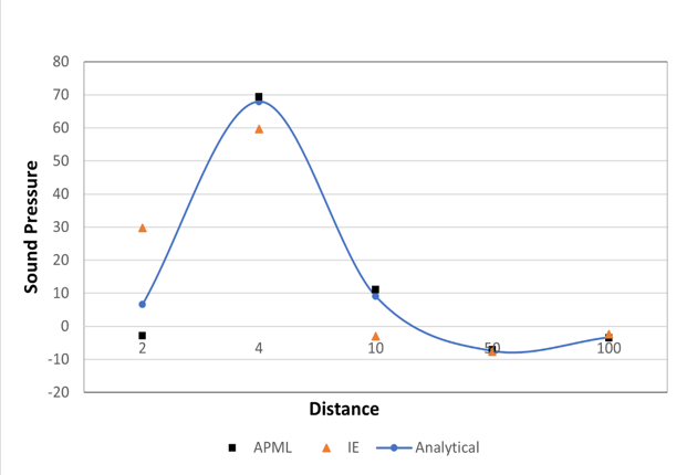

Figure 6. Imaginary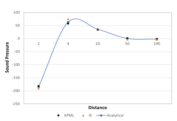
Microphone Sound Pressure versus Distance ( $k$ = 3)
Figure 7. Real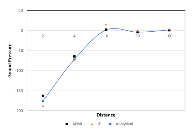

Figure 8. Imaginary

¹ Pierce, Allan D. Acoustics: An Introduction to Its Physical Principles and Applications. Springer, 2019