OS-E: 0320 Acoustic Analysis of a 2.1 Speaker using Infinite Elements
Demonstrate Infinite Elements, which is effectively modeled to measure the sound pressure of the 2.1 Home Theater System in OptiStruct with effective modeling practice.
Model Files
Model Description
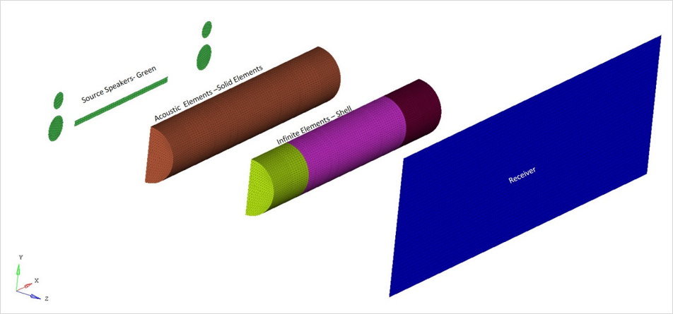
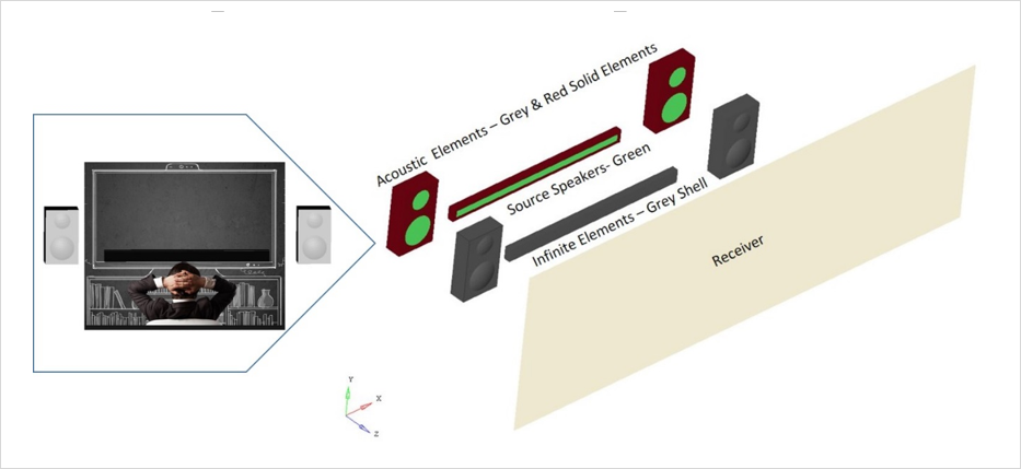
This example has a source plate (green in color) inside the speaker which is vibrating (unit displacement is applied as excitation) along the z-axis. The Source plates are then covered with acoustic fluid elements (front, back and top) as seen in Figure 1. Then the infinite elements are the skin of the front fluid elements whose normal must be pointing towards the receiver as shown, each speaker with IE will have their own pole (which is the center of the source) location. For pressure (as calculated on grids) contour, the receiver elements are configured with PLOTEL elements with fluid grids since you will be capturing the sound pressure on these elements. A direct frequency response analysis is run.
- Speakers
- First order Solid elements
- Source
- First order Shell
- Infinite Elements
- First order Shell
- Receiver
- First order Shell
- Property
- Value
- Young's Modulus
- 70000 MPa
- Poisson's Ratio
- 0.3
- Initial Density
- 2700 Kg/m3
- Property
- Value
- Speed of Sound
- 343 m/s
- Mass Density
- 1.21 Kg/m3
Results
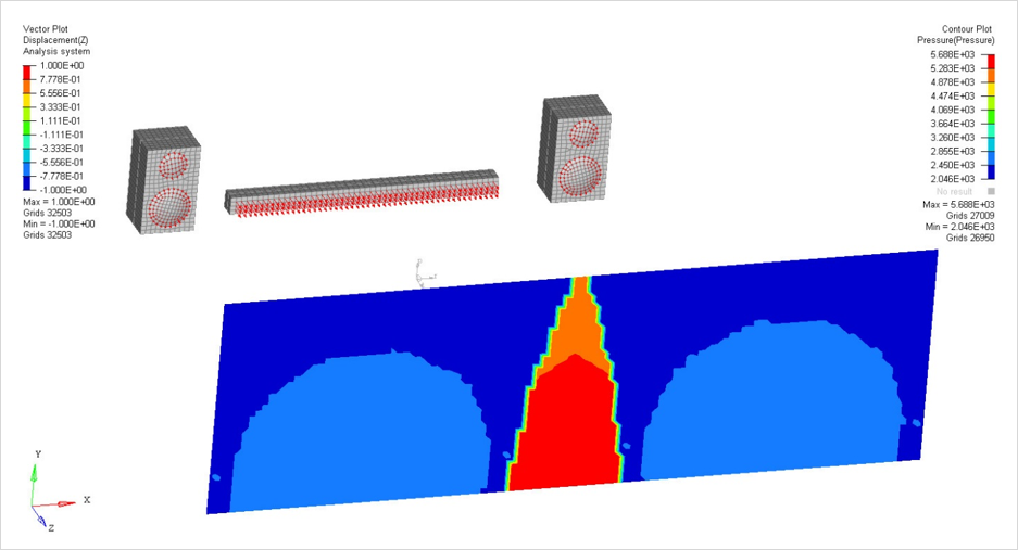
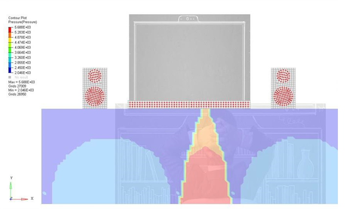
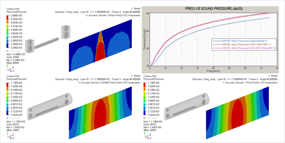
As you observer from the contour plot, the acoustic pressure is concentrated in the center along with the imprint of the left and right speaker, hence this does not capture the interaction of the 3 source speaker correctly due to incorrect modeling.