MV-1020: Model 2D Rigid to Rigid Contact Simulation
Tutorial Level: Intermediate Learn how to create Curve Entities and Curve Graphics, use macros to create them
simultaneously, and setup a 2D rigid curve to curve contact.
This tutorial will guide you through the 2D rigid body contact capabilities in
MotionSolve. This can be used when contact occurs in a
plane. You will model a roller type cam-follower mechanism using 2D rigid to rigid
contact as there are no out-of-plane contact forces that are expected.Figure 1.
Review the Model
Review the model by running it using MotionSolve.
Copy the files Cam_Follower_Input.mdl,
CamProfile.h3d, Cam_Fixed.csv and
Cam_Variable.csv from the location
<installation_directory>\tutorials\mv_hv_hg\mbd_modeling\interactive\
to your <working directory>.A partially setup model is available for you in MotionView. Everything except for the 2D contact has been setup.
Launch MotionView.
Open the Model by doing one of the following:
On the Standard toolbar, click (Open Model).
On the menu bar, click File > Open > Model.
From the Open model dialog, select the file
Cam_Follower_Input.mdl from your working directory
and click Open.
Review the model for its bodies, graphics, markers, joints, and motion. It
will look like the image in Figure 2.Figure 2.
Click the (Run panel) icon.
Click the Save and run current model browser button.
Then click the Run
button.
Once the simulation is completed, close the solver window and the
Message Log.
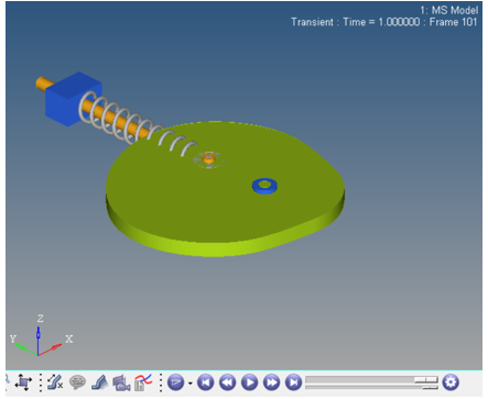
From the Run panel, review the results animation by clicking on the
Animate button.
Notice that the FollowerRoller is not in contact with the Cam since there is
no contact defined in the model.Figure 3.
Click the (Page Window Layout) button to return to the
MotionView window.
Figure 4.
Create Curve Entity and Curve Graphics
Create the Curve Entity and Curve Graphics for FollowerRoller.
Since the FollowerRoller profile is circular, it can be easily defined using
mathematical expressions. First, you will create a closed circular Curve Entity (using
the Math option). Next you will create Curve Graphics to associate this Curve Entity
with the FollowerRoller body so you can use it to setup the 2D Contact.
Open the Add Curve dialog by doing one of the
following:
From the Project Browser, right-click on
Model and select Add > Reference Entity > Curve.
On the Reference Entity toolbar, click the (Curves) icon.
In the dialog, for Label enter Roller_Curve. For
Variable, enter crv_roller.
Click OK.
Figure 5.
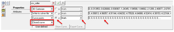
From the Properties tab, use the first drop-down menu to change the curve to
3D Cartesian.
Note: Only 3D Cartesian types of Curve Entities are supported for the Curve
Graphics.
Use the fourth drop-down menu to change the curve from Open Curve to
Closed Curve.
Click the x radio button, then select
Math from the second drop-down menu.
In the Expression Builder, enter 5*SIN(2*PI*(0:1:0.01)).
Then hit Enter.
For the Math expressions of the y and z coordinates, enter
5*COS(2*PI*(0:1:0.01)) and
0.0*(0:1:0.01) respectively.
Figure 6. You have finished creating the Curve Entity. Next, you will create a
graphic to represent the FollowerRoller body. Later, you will use this to define
2D Contact.
Open the Add CurveGraphic dialog by doing one of the
following:
From the Project Browser right-click on
Model and select Add > Reference Entity > Graphic.
On the Reference Entity toolbar, click the (Graphics) icon.
In the drop-down menu, choose Curve.
In the dialog, for Label enter Roller_Curve. For
Variable, enter gcrv_roller.
Click OK.
Figure 7.
Note: The Body/Point option (Parent type) has been selected by default on the
Connectivity tab.
From the Connectivity tab, double-click on the
collector. In the dialog, select FollowerRoller.
The collector is highlighted by default.
Click the collector. In the dialog, select
FollowerRevJoint.
Click the collector. In the dialog, choose
Roller_Curve. Leave the rest of the options on the
panel as default.
Figure 8.
Curve Graphics representing the FollowerRoller should now be graphically
visible.Figure 9.
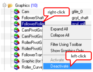
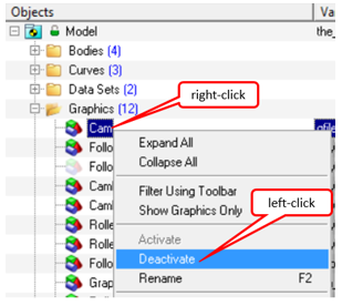
Now that you have created new graphics, deactivate the original cylinder
graphics used to represent the FollowerRoller.
In the Project Browser, right-click on
FollwerRoller.
In the context menu, click
Deactivate.
Figure 10.
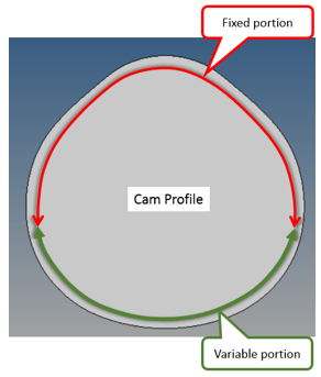
Create Curve Entity and Curve Graphics for Cam
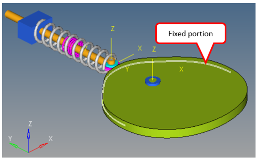
Divide the cam profile into Fixed and Variable portions to determine the best shape
of the cam for achieving a specific displacement profile of the follower.
Figure 11.
The variable portion of the cam will be controlled by the coordinates of some points
in the model.
Create Fixed Portion of Cam Profile
Use a .csv file containing x, y, and z coordinates of points to
create a Curve Entity.
Open the Add Curve dialog by doing one of the
following:
From the Project Browser right-click on
Model and select Add > Reference Entity > Curve.
On the Reference Entity toolbar, click the (Curves) icon.
In the dialog, for Label enter Cam_fixed_Curve. For
Variable, enter crv_cam_fix. Then click
OK.
From the Properties tab, use the first drop-down menu to change the curve to
3D Cartesian.
Verify the fourth drop-down menu selection is set to Open
Curve.
From the Properties tab, click on the x radio button.
Retain the default File option in the second drop-down menu.
Click and select Cam_Fixed.csv from the <working
directory>.
Click Open.
For component, select Column 1. Retain all other values
in the panel as default.
Figure 12.
For the y and z radio buttons, for Component select Column
2 and Column 3 respectively.
Create a Curve Graphic to visualize the cam and make sure the import data is
located as per your requirements.
Curve Graphics representing the fixed portion of Cam should now
be visible.Figure 14.
Create Variable Portion of Cam Profile
Use a macro to automatically create both the Curve Entity and Curve Graphics using
the existing points in the model.
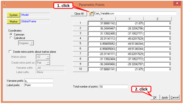
Create points for the model in one of the following ways:
From the menu bar, click Macros > Create Points > Using Coordinates.
On the MotionView Toolbar, click (Create Points using Coordinates).
In the Parametric Points dialog, click the (file
browser).
Select the Cam_Variable.csv and click
Open.
Click OK to create 10 points
(0 through 9).
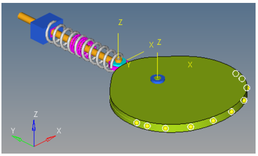
Figure 15 shows the newly
created points.Figure 15.
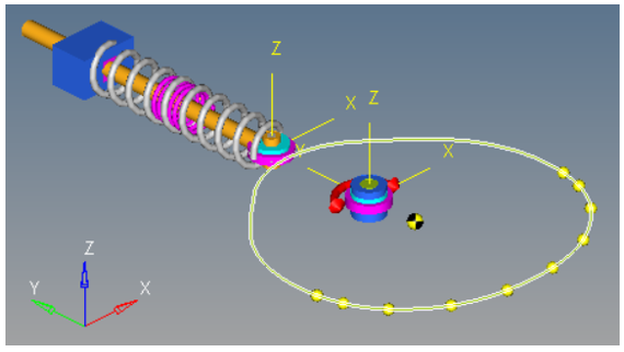
Now that you have created new graphics, deactivate the original H3D file
graphics used to represent the Cam.
In the Project Browser, right-click on
Cam.
In the context menu, click
Deactivate.
Figure 16.
.
Now use the newly created points to create the variable portion of
the cam profile using the Create Curve from Points/Nodes macro.
Open the Create Curve from Points/Nodes macro in one of
the following ways:
From the menu bar, click
MacrosCreate Curve from Points/Nodes/Edges/Faces.
On the MotionView toolbar, Click (Create Curve from Points/Nodes
button).
Figure 17.
Double-click the collector and select Cam
body.
Edit the Labels prefix for the Curve Entity and the Curve Graphics to be
created to Cam_Variable_Curve.
For the collector, select Point 0 in
one of the following ways:
Click Point 0 in the modeling window.
Click the collector. In the Select a
Point dialog, double-click on Point 0
from the filtered list of points.
Point 0 is highlighted in the modeling window and listed in the
panel.
Repeat step 9 to pick the
remaining points (1 through 9).
The panel should look as shown in Figure 18.Figure 18.
Note: A node associated with File graphic H3D can also be picked. However,
the curve created would not be parametrically linked with the node. Picking
a point retains the parametric relation between the point and the
curve.
Click Create.
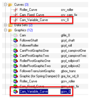
A new Curve Entity and a new Curve Graphics (Cam_Variable_Curve) has
been added to the model.Figure 19. The newly created Curve Graphics representing the variable portion of the
Cam should now be visible in the modeling window.Figure 20.
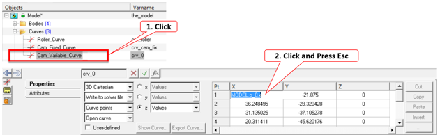
Review the newly created Curve Entity by selecting it from the Model Tree in the Model Browser.
Note: Click (as shown in Figure 21) to see how the X, Y and Z values in the panel are
parametrically pointing to the points selected while using the macro. Thus,
by changing the coordinates of these Points in the model, the curve can be
modified.Figure 21.
Create Merged Curve of Cam Profile
Merge both fixed and variable portions of the Cam and create a new closed curve to
setup the 2D Contact.
The fixed and variable Curve Graphics of Cam generated in Step 3.1 and Step 3.2
cannot be used in setting up contact since they are using open Curve Entities. You
generated these in order to verify if the curve data is in the correct location. For a
continuous contact between FollowerRoller and Cam, you need closed curves. In this step
you will merge the fixed and variable portions of the Cam and, in the process, learn how
to use a mathematical function (CAT) to concatenate two Curve Entities.
From the Properties tab, click the x radio button, then
select Math from the second drop-down menu.
In the Expression Builder, enter {CAT(crv_cam_fix.x,
crv_0.x)}. Then hit Enter.
For the Math expressions of the y and z coordinates, enter
{CAT(crv_cam_fix.y, crv_0.y)} and
{CAT(crv_cam_fix.z, crv_0.z)} respectively.
Note: By using CAT function, you are able to append the data-points of
variable portion of cam to the data-points of fixed portion of cam. The
panel should display merged data of both fixed and variable portions of cam
profile.Figure 22.
You have finished creating the Curve Entity. Next, you will
create a graphic to represent the Cam body. Later, you will use this to define
2D Contact.
Open the Add CurveGraphic dialog by doing one of the
following:
From the Project Browser right-click on
Model and select Add > Reference Entity > Graphic.
On the Reference Entity toolbar, click the (Graphics) icon.
In the drop-down menu, choose Curve.
In the dialog, for Label enter Cam_Curve. For Variable,
enter gcrv_cam.
Click OK.
Note: The Body/Point option (Parent type) has been selected by default on the
Connectivity tab. For this process you will use the Marker option since you
already have a CamMarker in the model which is associated with Cam (Body)
and PivotPoint (Point).
From the Connectivity tab, select the drop-down menu of
Parent and change it to
Marker.
Double-click on the collector.
In the Select a Marker dialog, select
CamMarker and click OK.
Double-click on the collector.
In the Select a Curve dialog, select
Cam_Curve.
Figure 23. The Curve Graphics representing the Cam should now be visible in the
modeling window.Figure 24.
Set Up 2D Contact
Define a contact between Cam and FollowerRoller using their respective Curve
Graphics.
On the Force Entity toolbar, right-click on the (Contact) button.
In the dialog, for Label enter 2D Contact 0 and retail
the default Variable.
In the drop-down menu, change the Type to 2D Rigid to
Rigid and click OK.
Figure 25.
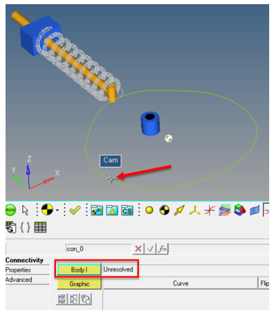
In the Connectivity tab, click the
(I Body) collector. Then select the Cam body by clicking
its Curve Graphics in the modeling window.
Figure 26.
(J Body) collector is highlighted
automatically.
Click the collector and select the
FollwerRoller body in the dialog.
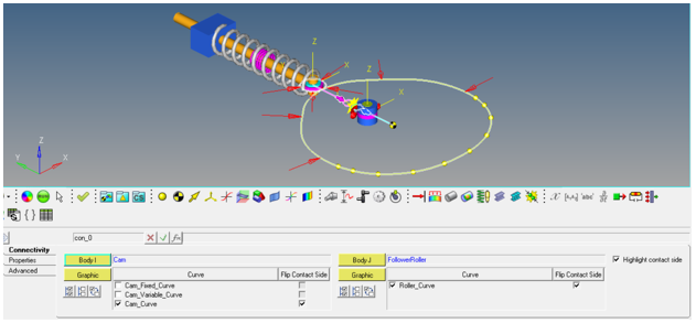
The Contact panel should now appear as shown in Figure 27:Figure 27.
Note: Fixed and Variable Curve Graphics are selected by default since they
are associated with Cam body. You can remove the same from the contact
definition as they are not required.
Under , deselect (or uncheck)
Cam_Fixed_Curve and
Cam_Variable_Curve.
Review the side of selected curves that will be in contact.
Click to check the Highlight contact side check
box.
Note: The arrow display indicates the inside of Cam and FollowerRoller
as contacting side. This needs to be corrected.
For both and curves, click to check the Flip
Contact Side box.
Note: The highlighted contact side for both the bodies should now be as
shown in Figure 28:Figure 28.
In the Properties tab, retain the default selections.
In the Advanced tab, activate the Find precise contact
event and Change simulation max step size
options with the default values.
Save and Run the Model
Save the 2D Contact model and run it using MotionSolve.
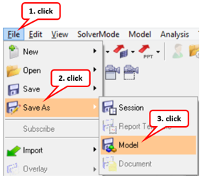
From the menu bar, click File > Save As > Model.
Figure 29.
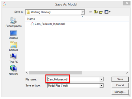
In the dialog, browse to your <working directory> and
specify the file name as Cam_Follower.mdl.
Figure 30.
Run the model.
A 2D curve contact simulation should run faster than an equivalent model using
3D contact where the solver must work harder to determine contact for a 2D
tessellated geometry.
Click the (Run panel) icon.
Note: To obtain accurate results, a smaller step size and a finer print
interval have been selected in this model. You can review them by
clicking the Simulation Settings…
button.
Click the (file browser) and specify the new name for
the file as Cam_Follower.xml.
Click Save.
Figure 31.
Click the Run button.
Post-Process the Results
Review the MotionSolve simulation summary using HyperView and HyperGraph.
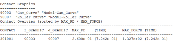
After the simulation is complete, MotionSolve prints
out a summary table like for 3D contact (both on screen-solver view window and in the
log file generated) that lists the contact pairs ordered by maximum penetration depth
and by maximum contact force for this simulation.Figure 32.
Click the Animate button to review the animation in
HyperView.
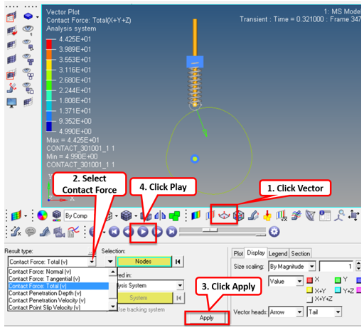
Review the contact force.
Select Vector plot.
Set the Results type to Contact Force.
Click Apply. Then
click (Start Animation).
Figure 33.
Plot the FollowerShaft vertical displacement during the entire simulation using
HyperGraph.
In the MotionView window, on the Run panel,
click the Plot button.
This will open an .abf file in HyperGraph.
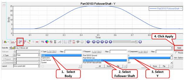
Click (Build Plots).
For Y Type (Axis), select Body. For Y Request,
select FollowerShaft. For Y Component, select
Y.
Click Apply.
Figure 34.
Optional: In MotionView, edit the coordinates of any/all
points (Point 0 to Point 9) to get updated Cam profile and re-run the model to
investigate its effect on Contact Force on Cam or FollowerShaft
Displacement.


 (Open Model).
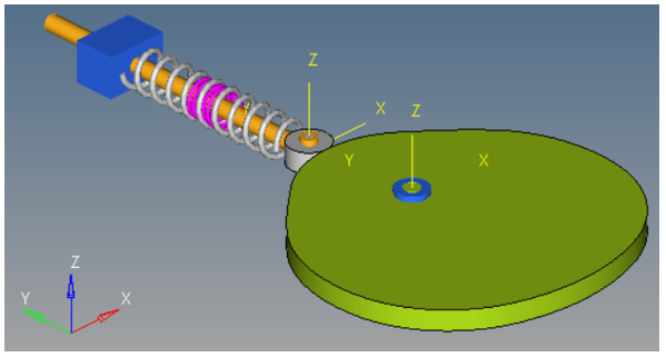
 (Run panel) icon.
 (Page Window Layout) button to return to the
MotionView window.
(Page Window Layout) button to return to the
MotionView window.

 (Curves) icon.
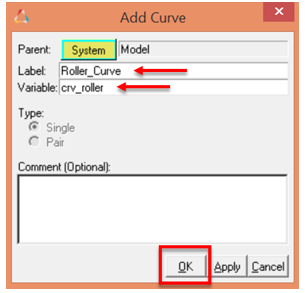
 (Graphics) icon.
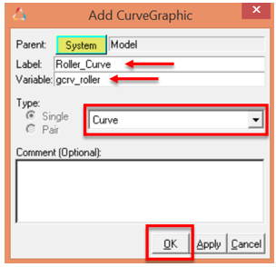 Note: The Body/Point option (Parent type) has been selected by default on the Connectivity tab.
 collector. In the dialog, select FollowerRoller.
The
collector. In the dialog, select FollowerRoller.
The collector is highlighted by default.
 collector. In the dialog, choose
Roller_Curve. Leave the rest of the options on the
panel as default.
collector. In the dialog, choose
Roller_Curve. Leave the rest of the options on the
panel as default.


 and select Cam_Fixed.csv from the <working
directory>.
and select Cam_Fixed.csv from the <working
directory>.


 (Create Points using Coordinates).
 (Create Curve from Points/Nodes
button).
(Create Curve from Points/Nodes
button).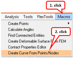
 collector, select Point 0 in
one of the following ways:
collector, select Point 0 in
one of the following ways:


 collector.

 (Contact) button.

 (I Body) collector. Then select the Cam body by clicking
its Curve Graphics in the modeling window.
(I Body) collector. Then select the Cam body by clicking
its Curve Graphics in the modeling window.
 (J Body) collector is highlighted
automatically.
(J Body) collector is highlighted
automatically.

 (Start Animation).
 (Build Plots).