
MV-7004: Inverted Pendulum Control Using MotionSolve and MATLAB
Tutorial Level: Advanced In this tutorial, you will learn how to use MotionView and MotionSolve to design a control system that stabilizes an inverted pendulum.
The goal of this tutorial is to design a regulator using the pole placement method. The inverted pendulum MDL model file is supplied.
- Check the stability of the open loop system.
- Export linearized system matrices A,B,C, and D using MotionSolve linear analysis.
- Design a controller using MATLAB.
- Implement a controller in MotionView.
- Check the stability of a closed loop system using MotionSolve linear analysis.
- Add disturbance forces to the model and run simulation using MotionSolve.
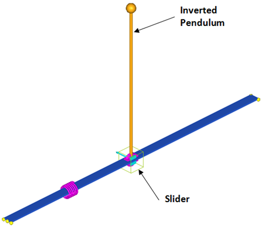
You want to find a full-state feedback control law to achieve the goal. The control input is a force applied to the slider along the global X-axis. Plant output is the pendulum angle of rotation about the global Y-axis.
Start by loading the file inv_pendu.mdl, located in the mbd_modeling\motionsolve folder, into MotionView. Upon examination of the model topology, you will notice that everything needed for this exercise is already included in the model. However, depending on which task you are performing, you will need to activate or deactivate certain entities.
Determine the Stability of the Open Loop Model
Compute the eigenvalues to determine the stability of the Inverted pendulum.
- From the Project Browser, click Forces and make sure that Control ForceOL is activated, while Control Force - CL and Disturbance-step are deactivated.
-
From General Actions toolbar, click Run
 .
.
- From the Simulation type drop-down menu, select Static + Linear.
- Specify the output filename as inv_pendu_ol_eig.xml.
- Select the MDL animation file (.maf) option.
- Click Run.
- Once the solution is complete, close the solver execution window and the message log.
The eigenvalues computed by MotionSolve are shown in the table below and can be viewed in the inv_pendu_ol_eig.eig file using a text editor.
Table 1. Open Loop Eigenvalues Number Real(HZ) IMAG_FREQ(HZ) 1 -1.625311E-02 0.00000000E+00 2 -4.003403E-01 0.00000000E+00 3 5.582627E-01 0.00000000E+00 4 -1.733216E+00 0.00000000E+00 There is one eigenvalue with a positive real part, indicating that the system is unstable in the current configuration.
-
Click Animate.
The result animation H3D will be loaded in the adjacent window.
-
From the Results Browser select individual modes.
Figure 2. 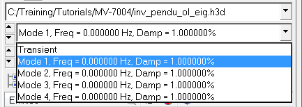
-
Click Start/Pause Animation
 to visualize the mode shape.
Obtain a Linearized Model
Usually, the first step in a control system design is to obtain a linearized model of the system in the state space form,
where , , , and are the state matrices, is the state vector, is the input vector, and is the output vector. The A,B,C,and D matrices depend on the choice of states, inputs, and outputs. The states are chosen automatically by MotionSolve and the chosen states are reported in one of the output files. You only need to define the inputs and outputs.
-
Expand the Solver Variables folder in the Project Browser and examine the entities.
- Control Force Variable - CL is used to define the control input after the control law has been found. Ignore this at this stage.
- Control Force Variable - OL is used to define the control plant input, which is a force named Control Force - OL. This force is applied to the slider body. This variable is set to zero. It is needed by MotionSolve to properly generate the linearized system matrices.
- Solver variable Pendulum Rotation Angle defines the control plant output and measures the pendulum rotation about the Global Y-axis.
-
Expand the Solver Array folder in the Project Browser and examine the solver arrays that are
defined.
-
Click Run
.
- From the Simulation type drop-down menu, select Linear.
-
Specify the output filename as
inv_pendu_state_matrices.xml.
Figure 3. Linear Tab in Simulation Settings Dialog for Specifying the MATLAB Matrix Files Output 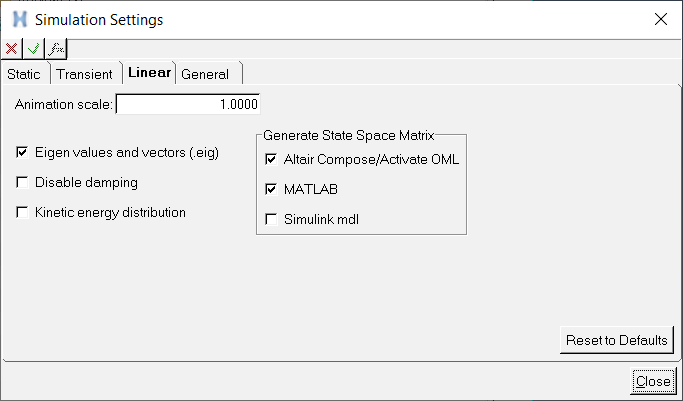
- From the Simulation Settings dialog, click the Linear tab and select the MATLAB option under the Generate State Space Matrix section.
-
From the Main tab, click Run.
You should get six new files with base name inv_pendu_state_matrices and extensions .a, .b, .c, .d, .pi, and .po. The .pi and .po files contain information about the input and output variables.
The states chosen by the MotionSolve solver are:
- Angular displacement about the global-Y axis.
- Translation displacement along the global X-axis.
- Angular velocity about the global-Y axis.
- Translation velocity along the global X-axis of the pendulum body center of mass marker.
Design a Control System in MATLAB
A detailed discussion of control system design is beyond the scope of this document. However, the steps to design a regulator using pole placement [1] to stabilize the inverted pendulum are described briefly. For details, refer to the standard controls text and the MATLAB documentation.
It can be easily verified using MATLAB that the system is completely state controllable [1, 2].
We employ a full-state feedback control law
, where
is the control input,
is the gain vector, and
is the state vector. Then, assuming the desired pole
locations are stored in vector
, you may use the pole placement method to compute
. For desired poles at [-20 -20 -20 -20] (rad/s), the
acker function in MATLAB yields k=1e3[-2.4186 -0.0163 -0.070
-0.0033].
Implement the Control Force in
`-1e3*(-2.4186*AY({b_pendu.cm.idstring})-0.0163*DX({b_pendu.cm.idstring}),-0.070*WY({b_pendu.cm.idstring})-0.0033*VX({b_pendu.cm.idstring}))`Notice that it is simply the dot product between the gain vector (k) and the state vector (x) elements. This solver variable is used to define a force named Control Force - CL.
Activate the force Control Force - CL if it is deactivated.
Check the Stability of a Closed Loop System
- From the SolverMode menu, select MotionSolve. Activate the force Control Force - CL if it is deactivated.
- From the Run panel, under Simulation type, select Linear.
-
Specify the output file as inv_pendu_cl_eig.xml and click
Run.
The eigenvalues are given below.
Table 2. Closed Loop Eigenvalues Number Real(cycles/second) Imag. (cycles/second) 1 -1.9595991E+00 2 -4.6976071E+00 3 -3.0372880E+00 +/- 1.3849641E+00 They all have negative real parts, hence the system is stabilized. Note that the negative real parts are close to the desired poles (-20 rad/s = -3.038 Hz).
Add Disturbance Force and Running the Simulation
-
Activate force acting on the slider titled
Disturbance-step, defined using a step
function:
Fx= `step(TIME,.1,0,.5,50) + step(TIME,1,0,1.5,-50)` Fy=0 Fz=0 - To run a dynamic simulation with MotionSolve, from the Project Browser, activate deactivated outputs Output control force - final and Output Disturbance step.
-
From the toolbar, click Run
.
- From the Simulation type drop-down menu, select Transient.
- Specify the output filename as inv_pendu_dyn.xml.
- Specify the End time and Print interval as 3.0 and 0.01, respectively.
- From the Main tab, click Run.
-
Once the job is completed, close the solver window and plot the following
results in a new HyperGraph page using
inv_pendu_dyn.abf.
Output Y-Type Y-Request Y-Component control force Marker Force REQ/70000014 Control Force - CL on Body slider(Output control force - final) FX disturbance force Marker Force REQ/70000017 Disturbance-step on Body slider(Output Disturbance step) FX slider displacement -X Marker Displacement REQ/70000006 Body slider(Output slider-disp) DX pendulum angular displacement Expressions REQ/70000016 Output Pendu rotation F2 The plots of disturbance force, control force, slider x displacement, and pendulum angular displacement are shown below.Figure 4. Plots of Disturbance and Control Forces as well as Slider Translational and Pendulum Angular Displacements 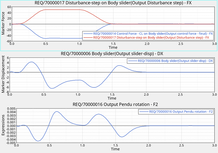
References
Feedback Control of Dynamic Systems, G. G. Franklin, J. D. Powell, and A. Emami-Naeini, Third Edition, Addison Wesley.