HS-5010: Reliability Analysis of an Optimum

In this tutorial, you will perform a reliability analysis to determine how sensitive the objective is to small parameter variations around the optimum.

Before you begin this tutorial, complete HS-1630: Set Up an Optimization Based on a Flux Application Example or import the archive file HS-1630.hstx from <hst.zip>/HS-1630/ to your working directory.

The objective has been minimized to superimpose the computed values to the reference.

In a Stochastic study, the parameters are considered to be random (uncertain) variables. This means parameters could take random values following a specific distribution (as seen in the normal distribution in Figure 1) around the optimum value (µ). The variations are sampled in the space and the designs are evaluated to gain insight into the response distribution.
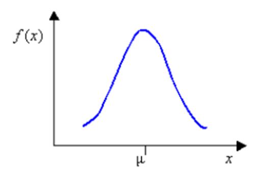
Figure 1.


Run Stochastic

In this step, you will check the reliability of the optimal solution found with GRSM. You will use Normal Distribution for the parameter variations and MELS DOE for the space sampling.

  1. Add a Stochastic.
    1. In the Explorer, right-click and select Add from the context menu.
      The Add dialog opens.
    2. For Definition from, select an approach.
    3. Select Stochastic, then Setup and click OK.
  2. Go to the Define Input Variables step.
  3. In the Nominal column, copy the parameter values at the optimal design.
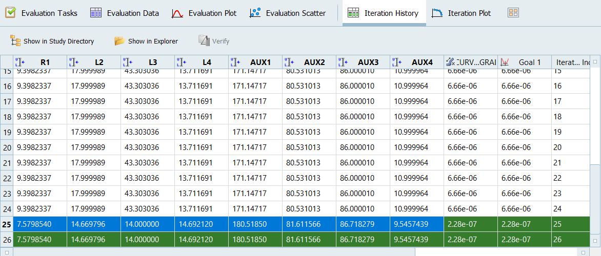
    1. Go to the GRSM_InclMatrix > Evaluate step. and copy the parameter values from the Iteration History tab.
    2. Go to the Iteration History tab and copy the optimal parameter values for R1 through AUX4 as show in Figure 2.
      Figure 2.


    3. Go to Stochastic 1 > Define Input Variables.
    4. Right-click on the header of the Nominal column and select Paste transpose from the context menu.
  4. Go to the Distributions tab.
    1. In the Distribution column, verify the distribution type is set to Normal Variance.

    For Stochastic studies, you must provide data about the standard variation σ MathType@MTEF@5@5@+= feaahqart1ev3aaatCvAUfeBSjuyZL2yd9gzLbvyNv2CaerbuLwBLn hiov2DGi1BTfMBaeXatLxBI9gBaerbd9wDYLwzYbItLDharqqtubsr 4rNCHbGeaGqiVu0Je9sqqrpepC0xbbL8F4rqqrFfpeea0xe9Lq=Jc9 vqaqpepm0xbba9pwe9Q8fs0=yqaqpepae9pg0FirpepeKkFr0xfr=x fr=xb9adbaqaaeGaciGaaiaabeqaamaabaabaaGcbaGaeq4Wdmhaaa@37B6@ (or variance σ 2 MathType@MTEF@5@5@+= feaahqart1ev3aaatCvAUfeBSjuyZL2yd9gzLbvyNv2CaerbuLwBLn hiov2DGi1BTfMBaeXatLxBI9gBaerbd9wDYLwzYbItLDharqqtubsr 4rNCHbGeaGqiVu0Je9sqqrpepC0xbbL8F4rqqrFfpeea0xe9Lq=Jc9 vqaqpepm0xbba9pwe9Q8fs0=yqaqpepae9pg0FirpepeKkFr0xfr=x fr=xb9adbaqaaeGaciGaaiaabeqaamaabaabaaGcbaGaeq4Wdm3aa0 baaSqaaaqaaiaaikdaaaaaaa@389F@ ) of parameters to account for uncertainties. This data should be defined in the 2 column of the Distributions tab. By default, σ 2 MathType@MTEF@5@5@+= feaahqart1ev3aaatCvAUfeBSjuyZL2yd9gzLbvyNv2CaerbuLwBLn hiov2DGi1BTfMBaeXatLxBI9gBaerbd9wDYLwzYbItLDharqqtubsr 4rNCHbGeaGqiVu0Je9sqqrpepC0xbbL8F4rqqrFfpeea0xe9Lq=Jc9 vqaqpepm0xbba9pwe9Q8fs0=yqaqpepae9pg0FirpepeKkFr0xfr=x fr=xb9adbaqaaeGaciGaaiaabeqaamaabaabaaGcbaGaeq4Wdm3aa0 baaSqaaaqaaiaaikdaaaaaaa@389F@ is computed in HyperStudy using the range rule σ 2 = ( U p p e r B o u n d L o w e r B o u n d ) 4 2 MathType@MTEF@5@5@+= feaahqart1ev3aaatCvAUfeBSjuyZL2yd9gzLbvyNv2CaerbuLwBLn hiov2DGi1BTfMBaeXatLxBI9gBaerbd9wDYLwzYbItLDharqqtubsr 4rNCHbGeaGqiVu0Je9sqqrpepC0xbbL8F4rqqrFfpeea0xe9Lq=Jc9 vqaqpepm0xbba9pwe9Q8fs0=yqaqpepae9pg0FirpepeKkFr0xfr=x fr=xb9adbaqaaeGaciGaaiaabeqaamaabaabaaGcbaGaeq4Wdm3aa0 baaSqaaaqaaiaaikdaaaGccqGH9aqpdaqadaqaamaalaaabaGaaiik aiaadwfacaWGWbGaamiCaiaadwgacaWGYbGaamOqaiaad+gacaWG1b GaamOBaiaadsgacqGHsislcaWGmbGaam4BaiaadEhacaWGLbGaamOC aiaadkeacaWGVbGaamyDaiaad6gacaWGKbGaaiykaaqaaiaaisdaaa aacaGLOaGaayzkaaWaa0baaSqaaaqaaiaaikdaaaaaaa@519E@ which is a function of the DVs bounds. When you do not have reliable data about the standard deviation, you can modify the default σ 2 MathType@MTEF@5@5@+= feaahqart1ev3aaatCvAUfeBSjuyZL2yd9gzLbvyNv2CaerbuLwBLn hiov2DGi1BTfMBaeXatLxBI9gBaerbd9wDYLwzYbItLDharqqtubsr 4rNCHbGeaGqiVu0Je9sqqrpepC0xbbL8F4rqqrFfpeea0xe9Lq=Jc9 vqaqpepm0xbba9pwe9Q8fs0=yqaqpepae9pg0FirpepeKkFr0xfr=x fr=xb9adbaqaaeGaciGaaiaabeqaamaabaabaaGcbaGaeq4Wdm3aa0 baaSqaaaqaaiaaikdaaaaaaa@389F@ by modifying the upper and lower bounds of the parameters, as is done in step 5.

  5. Go to the Bounds tab.
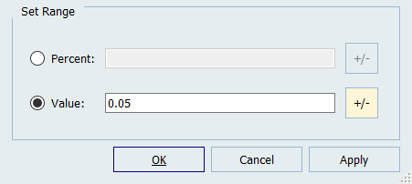
    1. For all active input variables, click (...) in the Nominal field.
    2. In the pop-up window, Value field, enter 0.05 and click +/-.
      Figure 3.


    3. Click OK.
    The values in the 2 column (variance) of the Distributions tab are updated.
  6. Go to the Specifications step.
    1. In the work area, set the Mode to Mels.
    2. Click Apply.
  7. Go to the Evaluate step.
    1. Click Evaluate Tasks.

Post-Process Stochastic Results

In this step, you will review the evaluation results within the Post-Processing step.

  1. Go to the Post Processing > Integrity tab.
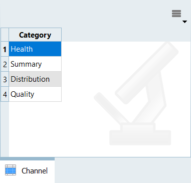
    1. Using the Channel selector, select the Health category to get a summarized view of statistics and spot eventual, missing, or bad values.
      Figure 4.


    2. Using the Channel selector, select the Summary category to get basic statistics information on the data.
      The Range column is useful in understanding the distribution of values in the data from the minimum to the maximum. The high spread of the response values in the Range column indicates a large disparity between the Minimum and Maximum values within the set of evaluations.
    3. Using the Channel selector, select the Quality category to recognize eventual outliers.
  2. Optional: Review evaluation fluctuations.
    1. Go to Evaluate > Evaluation Plot tab.
    2. Using the Channel selector, select the CURVE_DIFF_INTEGRAL label.
  3. Review the historgrams of the Stochastic results
    1. Go to the Post Processing > Distribution tab.
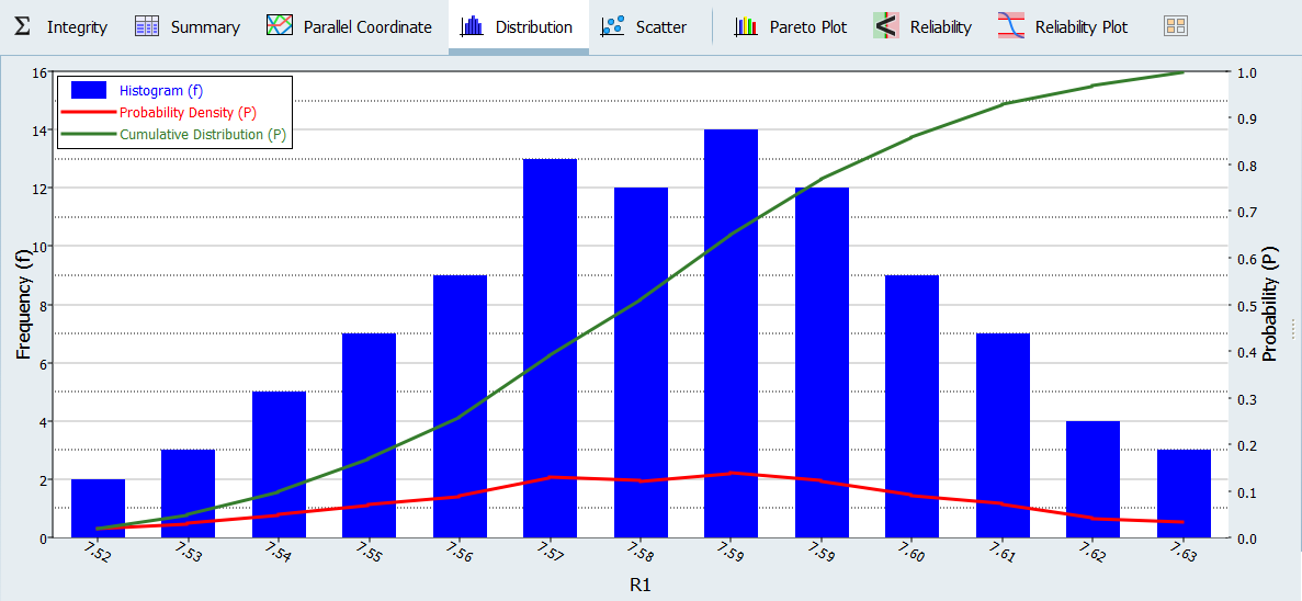
    2. Using the Channel selector, select R1.
      The chart in Figure 5 shows three pieces of information about the distribution of values for R1. The histogram uses the y-axis and represents the frequency of runs yielding a sub-range of response values. The probability density uses the x-axis, and indicates the relative likelihood of the variable to take a particular value. A high probability density indicates that the values are more probable to occur. The cumulative distribution uses the x-axis, and is equal to the integral of the probability density. The cumulative distribution value indicates what percentage of the data falls below the value’s threshold.
      Figure 5.


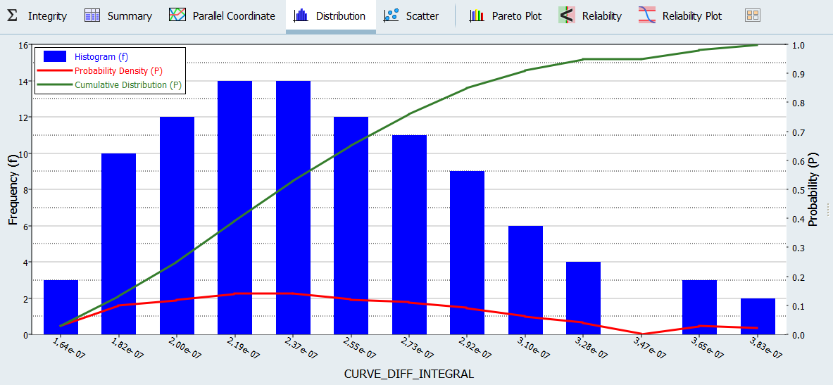
    3. Using the Channel selector, select CURVE_DIFF_INTEGRAL.
      A high frequency of runs yields a high probability density for this response value.
      Figure 6.


    4. Click and identify the outliers identified in step 1.b.
  4. Click the Pareto Plot tab.
    1. From the Channel selector, select Options.
    2. Enable the Effect curve checkbox.
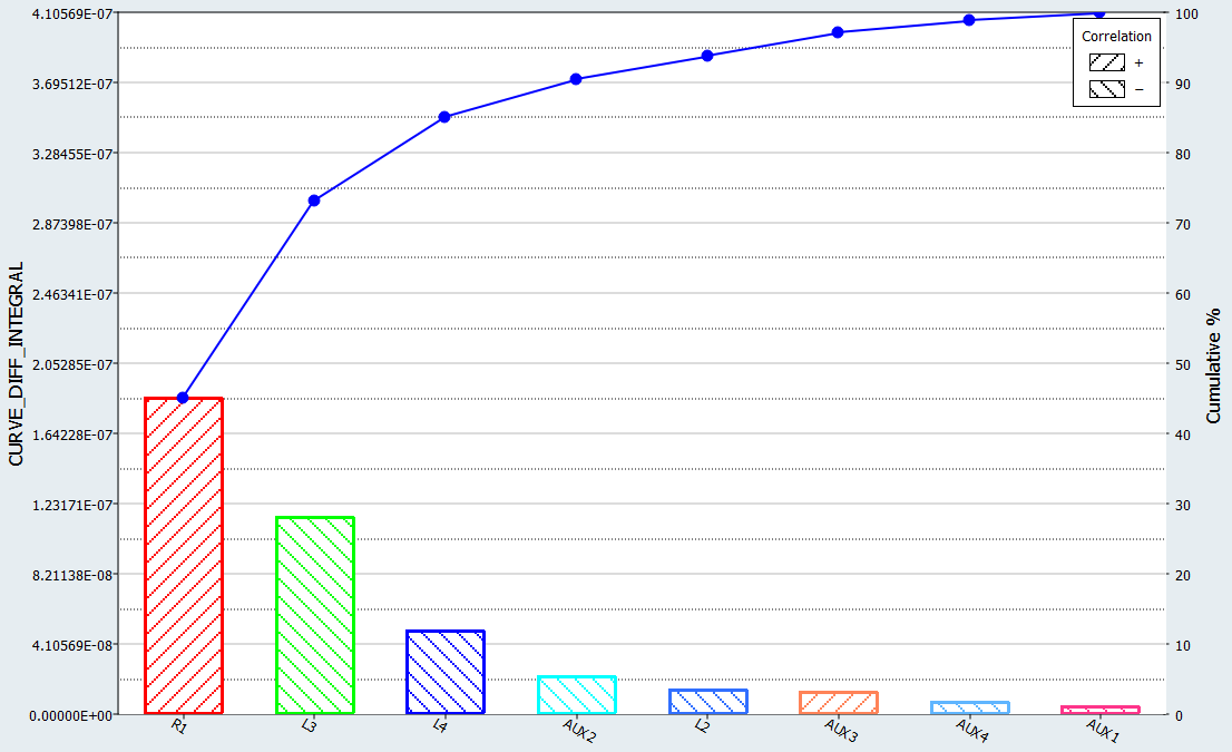
    The dashed lines indicate the effect. For example, R1 has a positive effect on the response meaning the response increases higher than the optimum for R1 values. A high response value means worse matching between the computed and reference curves.
    Figure 7.


  5. Estimate the probability of failure for the output responses (probability for an output response to violate a user selected bound).
    1. Click the Reliability tab.
    2. Click Add Reliability.
    The bound value is chosen with respect to the most probable value the response would take. It is higher than the optimum, but remains satisfactory as it still ensures good curves matching.