Input Variable Properties

In the Define Input Variables step, various input variable properties can be modified from the Bounds, Modes, and Distributions tabs.

Bounds

Lower bound: Lower limit of the variable range to be studied.
Nominal: Default value of the variable if deactivated; also serves as the initial value in an Optimization.
Upper bound: Upper limit of the variable range to be studied.

Data Type

Numeric: Variable stored as numerical value.
String: Variable stored as a character without any numeric meaning.

Format

Continuous: Input variable that can take any value between the lower and upper bounds, for example 1 < x < 2.
Fixed Precision: This controls the number of digits on the right side of decimal point. For example, if precision is set to 2 for 1.478, the outcome becomes 1.47.
Format Descriptor: This option controls the total number of digits and decimal point of values between lower and upper values. For example, for 0 < x < 1, %0.2f will produce values like 0.11, 0.23, 0.37, etc.
Step: This produces ordered values between lower and upper bounds based on user-defined step size. For example, 0 < x < 1, step size = 0.2 will produce values of 0.0, 0.2, 0.4, 0.6, 0.8, 1.0.
List: Input variable that can take values from a non-ordered list of values, for example x = red, green, blue or 3, 2, 7, 11.

Note: HyperStudy Format specifications are based on formatting schemes in C++ language.

Distribution

Input variables can be statistically characterized using various probability distributions. In statistical terms, an input variable is referred to as a random variable. While the term "random variable" may imply unpredictability in everyday language, in statistics it refers to a variable whose possible values and associated probabilities are known.

Input variables exhibit different properties depending on the parameter they represent. Some may be symmetrically distributed around the mean, while others may be skewed to the left or right. Variables can also be either bounded (limited to a specific range) or unbounded.

Variability in input variables falls into two categories: controllable and random. Controllable variability refers to variation within a known range, such as a sheet metal thickness of 6 ± 0.3 mm. In contrast, random variability (also called noise) is uncontrollable, such as fluctuations in wind speed during an open-air test.

Random variables can be continuous or discrete. A continuous random variable can assume any value within a given interval, while a discrete random variable can take only a finite set of values.

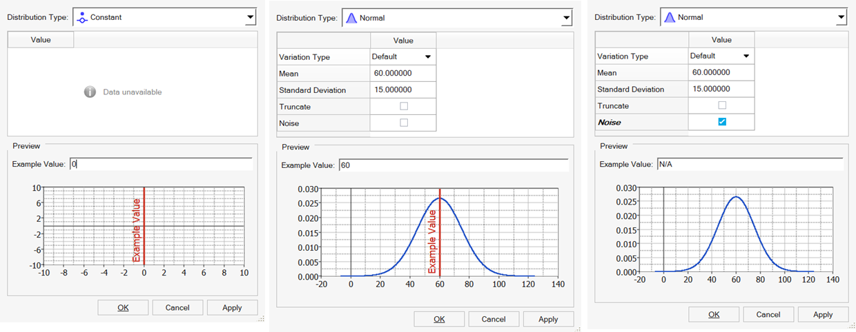
HyperStudy supports various types of distribution schemes. The most commonly used is the normal (Gaussian) distribution, where values are symmetrically distributed around an expected (mean) value. This expected value is often derived from an optimization process or trade-off study. Variation around the mean can be described using one of three measures: variance, standard deviation, or coefficient of variation.

In some cases, a variable may have no variability and is defined as a constant. This type of variable typically takes on a value determined by an optimization process or trade-off study.

Figure 1. Variable with variation; Variable with known variation; Noise

Note: The Truncate option limits sampling to within specified lower and upper bounds. Values outside these bounds are excluded.

Note: Distributions are only applicable in Stochastic and Reliability-based Optimization approaches. In DOE and Sampling Fit approaches, sampling is based solely on a uniform distribution.

Normal (CoV or Variance): Use to approximate many phenomenons in nature.
Figure 2.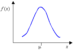

$f (x) = \frac{1}{\sqrt{2 Π σ^{2}}} e^{\frac{- {(x - μ)}^{2}}{2 σ^{2}}}$

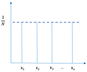
where $μ$ is the mean and $σ$ is the standard deviation.; In HyperStudy a normal distribution can be defined using mean, $μ$ and variance, $σ^{2}$ or using mean, $μ$ and coefficient of variance (CoV), $σ$ / $μ$ .; Variance is the second statistical moment and measures the spread of a distribution. CoV measures the relative spread of a distribution. The higher the CoV, the higher the variability.
Uniform: Use when all values between the minimum and maximum are equally likely, such as a number from a random number generator.
Figure 3.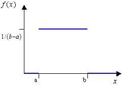

$\begin{array}{l} f (x) = {\begin{matrix} \begin{matrix} \frac{1}{b - a} \\ 0 \end{matrix} & \begin{array}{l} i f a \leq x \leq b \\ o t h e r w i s e \end{array} \end{matrix} \\ F (x) = {\begin{matrix} \frac{\begin{matrix} 0 \\ x - 1 \end{matrix}}{\begin{matrix} b - a \\ 1 \end{matrix}} & \begin{array}{l} i f x < a \\ i f a \leq x \leq b \\ i f x > b \end{array} \end{matrix} \end{array}$

where $a$ and $b$ are end points.
Triangular: Use when the only known information is the minimum, the most likely, and the maximum values.
Figure 4.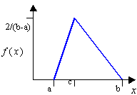

$f (x) = {| \begin{matrix} \frac{2 (x - a)}{(b - a) (c - a)} & i f a \leq x \leq c \\ \frac{2 (b - x)}{(b - a) (b - c)} & i f c \leq x \leq b \\ 0 & o t h e r w i s e \end{matrix}$

$F (x) = {\begin{matrix} 0 & i f x < a \\ \frac{{(x - a)}^{1}}{(b - a) (c - a)} & i f a \leq x \leq c \\ 1 - \frac{{(b - x)}^{1}}{(b - a) (b - c)} & i f c < x \leq b \\ 1 & i f b < x \end{matrix}$

where $a$ , $b$ , and $c$ are the end points and the mode.
Exponential: Use to describe the amount of time between occurrences, mean time between failures.
Figure 5.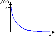

$\begin{array}{l} f (x) = {\begin{array}{l} λ e^{- λ x} & x \geq 0, \\ 0 & x < 0. \end{array} \\ F (x) = {\begin{array}{l} 1 - e^{- λ x} & x \geq 0, \\ 0 & x < 0. \end{array} \end{array}$

where $λ$ is the scale parameter.
Weibull: Principal applications are situations involving wear, fatigue and failure, failure rates, life-time expectancies.
Figure 6.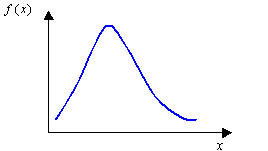

$f (x) = {\begin{matrix} {α β^{- α} x^{α - 1} e}^{- {(\frac{x}{β})}^{α}} & i f x > 0 \\ 0 & o t h e r w i s e \end{matrix}$

$F (x) = {\begin{matrix} 1 - e^{- {(\frac{x}{β})}^{α}} & i f x > 0 \\ 0 & o t h e r w i s e \end{matrix}$

where $α$ and $β$ are shape and scale parameters which enable it to be adjusted to desired fatigue or reliability laws.
Log Normal: Use in risk analyses.
Figure 7.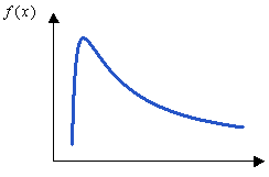

$f (x) = \frac{1}{x s \sqrt{2 π}} e^{\frac{- {(1 n x - m)}^{2}}{2 s^{2}}}$

where $m$ and $s$ are location and scale.
Uniform Discrete: Use when you have discrete (numeric or string) variables that take values which are equally likely.; Possible numeric values are 1, 2, 3, or 4; each are equally likely.; Possible string variables are orange, green, red, or blue; each are equally likely.; Figure 8.

$f (x) = \frac{1}{N} \forall x \in {x_{1}, x_{2}, ... x_{n}}$