Methods to Determine Elementary Material Block Size ρ*
Method 1: Using Fatigue Limit and Threshold Stress Intensity Range
This method requires knowledge of the fatigue limit and the threshold stress
intensity range. It was postulated in this method that the fatigue crack would not
grow under the applied stress intensity ranges equal to or less than the threshold
stress intensity range, such as when . Therefore, the stress range over the first
elemental material block at the crack tip should be simultaneously equal to or less
than the fatigue limit (that is, ). Since the fatigue limit () is less than the yield limit, only the linear
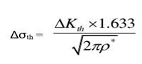
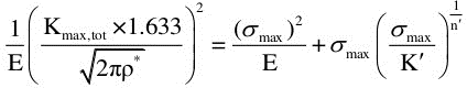
elastic analysis is required. According to the Creager-Paris solution the two
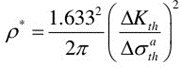
material properties can be related as:Figure 1. The elementary material block size, , can subsequently be expressed as:Figure 2.
This method provides a relationship between the elementary material block size and
fatigue properties of the material. Unfortunately, it requires a very accurately
determined threshold stress intensity range and fatigue limit which are not always
readily available. Additional care must be also taken to ensure that the fatigue
limit and threshold stress intensity range are obtained under the same stress ratio
R. An additional ambiguity also arises from the fact that the stress intensity range
is not the only parameter driving fatigue cracks. It has been pointed out by
Vasudevan et. al. 4 that there are two different threshold parameters, namely the
maximum threshold stress intensity factor and the threshold stress intensity range
and both should be simultaneously exceeded for the crack to grow. Therefore it is
not certain which threshold should be used to determine the elementary material
block size.
Lastly, the method described above neither proves nor disproves whether the
elementary material block size, , is only a material constant or if it also depends
on the applied load and specimen/crack geometry. It must also be verified that the value obtained from Figure 2 does not depend on the stress ratio at which the fatigue crack growth threshold
and the fatigue limit were determined.
Method 2: Using the Experimental Fatigue Crack Growth Data Obtained at Various
Stress Ratios
Since the mean stress effect has been already accounted for by using the SWT fatigue
damage parameter, all experimental fatigue crack growth rate data points plotted as
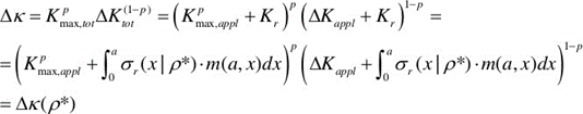
a function of the total two- parameter driving force, , should collapse onto one ’main’ curve. The total
two-parameter driving force, can be presented on the other hand as a function of
the elementary material block size, .Figure 3.
Where,
Residual stress intensity factor due to plastic deformaion
Residual stress
m
Weight function depending on crack geometry
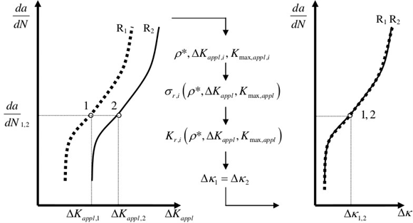
Since is the only unknown parameter in the equation above,
it has to be such that all experimental constant amplitude FCG data points obtained
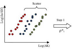
at various stress ratios R should collapse onto one vs. ‘main’ curve as shown in Figure 4.
Figure 4.
Constant amplitude fatigue crack growth data presented in terms of the applied stress
intensity range and the total driving force.
The ‘main’ curve shown in Figure 4 can be considered as theoretical idealization of the actual engineering model. In
practice, it would be a set of points deviating around some mean value due to the
natural scatter of the experimental fatigue crack growth data as shown in Figure 5.
Figure 5.
Figure 5 shows the initial FCG rate data without residual stress
effect. It is impossible to describe using only one 'main'
curve.
Figure 6.
Figure 6 shows the FCG rate data in terms of the total two-parameter
driving force corresponding to the first approximation of .
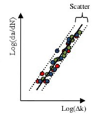
Figure 7.
Figure 7 shows the FCG rate data in terms of the total two-parameter
driving force with snakiest scatter.
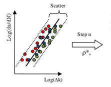
Iteration process for the elementary material block size estimation
based on Method 2 using linear ‘main’ curve.
Assuming some value of and performing all of the iterative steps (assume , find , find , and find ), it is possible to present FCG rate data in terms
of the total two-parameter driving force and fit by the mean (‘main') curve using
the least square method (Figure 6). However, the scatter of experimental FCG rate data shown in Figure 6 is relatively large. Therefore, the usual error minimization problem has to be
solved in order to find such elementary material block size, , that experimental FCG rates presented in terms of
corresponding driving force have the smallest scatter (Figure 7).
It should be mentioned that the method described above does not explicitly provide,
from the fatigue fracture point of view, information about the parameter as the elementary material block size. The parameter represents only an effective crack tip
radius subsequently influencing the magnitude and distribution for the residual
stress field.
It is also not clear whether the parameter is unique according to this method. The
method can be applied only if sufficient experimental fatigue crack growth data is
available (that is, constant amplitude data obtained at three stress ratios at least).
The advantage of using the method discussed in the current section is that parameters and in the crack growth equation shown in Figure 7 from the Crack Growth Mechanism page are determined from
experimental fatigue crack growth data and not from approximate expressions and
smooth specimen fatigue data. It is clear that, by fitting the and parameters into limited amount of experimental
fatigue crack growth data, the final equation simulates all other data much better
than the theoretically derived approximate formula shown in Figure 7 from Crack Growth Mechanism.
The collapsed experimental fatigue crack growth data is shown together with
analytical and fitted ‘main’ curves for the same . Since parameters ‘’ and ‘’ for analytical curve have been estimated in two
limited cases where either plasticity or elasticity effects were omitted, the curve
does not fit well the experimental FCG data in the region where both plasticity and
elasticity are important. Therefore, it can be concluded that the equation in Figure 7 from Crack Growth Mechanism provides only an empirical
relation between the instantaneous FCG rate and total SIFs. However, it is
preferable to fit parameters ‘’ and ‘’ based on the experimental FCG data.
Method 3: Using the Manson-Coffin Fatigue Strain-Life Curve and Limited Fatigue
Crack Growth Data
The procedure resulting in the determination of the parameter is summarized below.
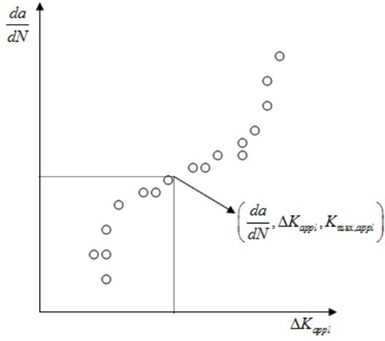
Assuming that experimental constant amplitude fatigue crack growth rate data, the
corresponding applied stress intensity ranges (Figure 8), and the stress ratio R are available, it is possible to determine the applied
stress intensity range and the maximum applied stress intensity factor for each
particular data point.
Figure 8.
Schematic of experimental fatigue crack growth rate data
As far as the stress state over the first elementary material block is concerned, it
can be noticed that there is only one non-zero stress component. Therefore, the
crack tip stress/strain analysis can be reduced to the uni-axial stress state.
The combination of the Ramber-Osgood material stress-strain
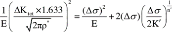
curve and the Neuber rule leads to the following equation:Figure 9. This equation makes it possible to determine the maximum elastic-plastic
stress over the first material block ahead of the crack tip as a function of the
applied maximum stress intensity factor. A similar equation can be obtained for the
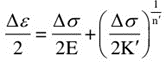
elastic-plastic stress range produced by the unloading reversal:Figure 10. The elastic-plastic strain range can be subsequently determined from the
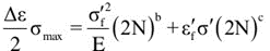
expanded by a factor of two cyclic stress/strain curves:Figure 11. Finally, the maximum stress and the actual strain range have to be combined
using the Smith-Watson- Topper (SWT) fatigue damage parameter in order to find the
number of cycles required to break the first elementary material block:Figure 12. The equations shown in Figure 6, Figure 9, Figure 10, Figure 11, and Figure 12 provide the solution to five unknown variables: , , , , and . Therefore, the elementary material block size can be determined for each particular point of the
experimental fatigue crack growth rate curve.
It is important to note that the equations in Figure 9 and Figure 10 contain the maximum total stress intensity factor and the total stress intensity
range, but not the applied ones. However, since the elementary material block size
and corresponding residual stresses are not known yet, the applied stress intensity
factors can be used only as the input for the first iteration.
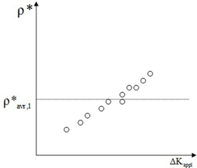
Subsequent solutions of the set of equations from Figure 6, Figure 9, Figure 10, Figure 11, and Figure 12 for each experimental FCG data point provide elementary material block sizes as a
function of the applied stress intensity ranges (Figure 13, Figure 14) corresponding to specific measured fatigue crack growth rates. It can be
observed that the elementary material block size is not constant and depends on the
load level. Therefore, it contradicts the basic assumption of the model that the parameter was supposed to be a constant parameter
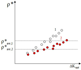
characteristic for a given material. The apparent dependence of the parameter on the load is the result of using applied
stress intensity factors in the set of equations from Figure 6, Figure 9, Figure 10, Figure 11, and Figure 12 without accounting for residual stresses induced in due course around the crack
tip. Therefore, residual stresses induced ahead of the crack tip during the first
iteration should be accounted for in the next iteration, resulting in a more
accurate estimation of the parameter. This means that, after the first
iteration, instead of being applied, the total stress intensity factors are used by
accounting for the residual stress obtained during the preceding
iteration.
Figure 13.
Figure 13 shows the elementary material block size as a function of the
applied stress intensity range after first iteration
Figure 14.
Figure 14 shows the elementary material block size as a function of the
applied stress intensity range after two iterations
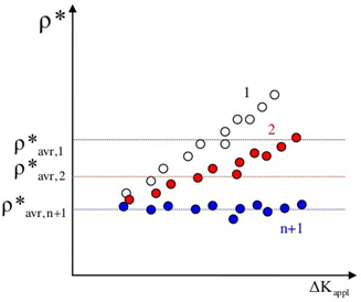
Figure 15.
Elementary material block size as a function of applied stress intensity
range after n+1 iterations when the convergence was reached
This way, new values of the parameter are obtained after each iteration. The
iteration procedure is complete when the same approximate value of the parameter is obtained for all experimental data
points.
Surprisingly, sometimes only two iterations are sufficient in order to obtain the
same value of the parameter for all experimental data points (that is, the value independent of the load configuration). The
iteration process must be repeated in practice as many times as it is necessary to
achieve some kind of convergence (see Figure 15) measured by the variation of individual of the average parameter in such a way that with required accuracy, where ‘n’ is the number of
iterations. The average value of the parameter is determined as the average of all
results obtained for the entire population of experimental data points.
The method described above requires solving the system of five simultaneous nonlinear
equations (see Figure 6, Figure 9, Figure 10, Figure 11, and Figure 12) for each experimental fatigue crack growth data point. The number of iterations
necessary for obtaining the converged value of the parameter usually ranges from five to 10 iterations.
The equation system can only be solved numerically. The method does not require
large amount of experimental data and sufficient estimation of the parameter can be obtained using only few data points
(>3)
It has been also shown that the elementary material block size obtained by the third
method does not depend on the stress ratio R. In other words, the same value of the parameter should be obtained regardless of the
stress ratio R at which the experimental constant amplitude fatigue crack growth
data was generated.