
ACU-T: 3204 Radiation Heat Transfer in a Simple Headlamp using the Discrete Ordinate Model
Tutorial Level: Intermediate
Prerequisites
This tutorial introduces you to setting up a radiation heat transfer problem using the Discrete Ordinate radiation model in HyperMesh CFD. Prior to starting this tutorial, you should have already run through the introductory tutorial, ACU-T: 1000 UI Introduction, and have a basic understanding of HyperMesh CFD and AcuSolve. To run this simulation, you will need access to a licensed version of HyperMesh CFD and AcuSolve.
Problem Description

| Absorption Coefficient | Refractive Index | |
|---|---|---|
| Air | 0 | 1.0 |
| Lens | 900 | 1.57 |
| Surface Type | Radiation Surface Type |
|---|---|
| Participating medium - Participating medium Interface | Radiation Interface - Internal |
| Participating medium - (Non- Participating) medium Interface | Wall |
| External boundaries of Participating medium | Radiation Interface - External or Wall |
Start HyperMesh CFD and Create the HyperMesh Model Database
-
Start HyperMesh CFD from the Windows Start
menu by clicking .
When HyperMesh CFD is loaded, the Geometry ribbon is open by default.
-
Create a new .hm database in
one of the following ways:
- From the menu bar, click .
- From the Home tools, Files tool group, click the Save As tool.
Figure 4. 
- In the Save File As dialog, navigate to the directory where you would like to save the database.
-
Enter Headlamp_DO as the name for
the database and then click Save.
This will be your problem directory and all the files related to the simulation will be stored in this location.
Import and Validate the Geometry
Import the Geometry
- From the menu bar, click .
- In the Import File dialog, browse to your working directory and then select ACU-T3204_headlamp.x_t and click Open.
-
In the Geometry Import Options dialog, leave all the
default options unchanged and then click Import.
Figure 5. 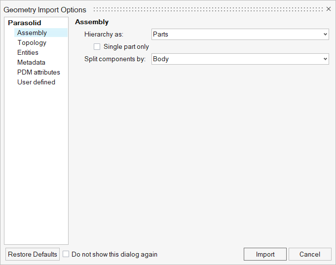
Figure 6. 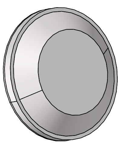
Validate the Geometry
-
From the Geometry ribbon, click the Validate tool.
Figure 7. 
The Validate tool scans through the entire model, performs checks on the surfaces and solids, and flags any defects in the geometry, such as free edges, closed shells, intersections, duplicates, and slivers.The surface and solid errors display in the list below the tool.Figure 8. 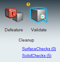
-
Click SolidChecks.
The Solid Repair tool opens, which you can use to fix the geometric errors in the model.From the SolidChecks legend, you can see the model's solids have five intersections.
Figure 9. 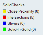
-
Click Intersections.
A guide bar used to fix intersecting solids displays.
- Optional:
Click
 and
and  to review each
error.
to review each
error.
-
Activate the Keep common interface option then click
Combine All.
The SolidChecks legend should now display zero for all errors.
-
Click the Validate tool
once again.
Observe that a blue check mark now appears on the top-left corner of the tool icon. This indicates that no issues are detected and you are ready to continue.
Figure 10. 
Set Up Flow
Set the General Simulation Parameters
-
From the Flow ribbon, click the Physics tool.
Figure 11. 
The Setup dialog opens. -
Under the Physics models setting:
- Verify that Time marching is set to Steady.
- Select Laminar as the Turbulence model.
- Activate the Include gravitational acceleration checkbox and set the gravity in the y direction to -9.81.
- Activate the Heat transfer checkbox.
Figure 12. 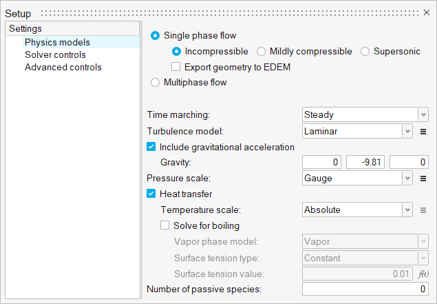
-
Click the Solver controls setting and activate the
Thermal flow equation.
Figure 13. 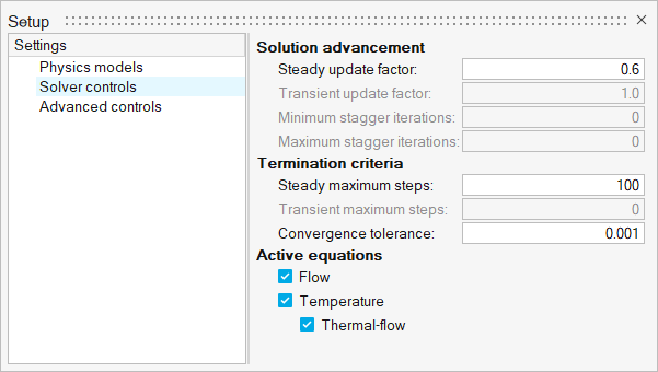
- Close the dialog and save the model.
Define the Material Models
-
From the Flow ribbon, click the Material Library tool.
Figure 14. 
The Material Library dialog opens. - Click the My Materials tab.
-
Click
 to add a new fluid
material model.
to add a new fluid
material model.
- In the material creation dialog, click the name in the top-left corner and rename the material to Air_Boussinesq.
-
In the Density tab,
- Set the Type to Boussinesq.
- Set the Density value to 1.225.
- Set the Expansivity value to 0.00347222.
- Reference temperature value to 288.
Figure 15. 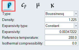
-
Click the Specific Heat tab and set the Specific heat
value to 1005.
Figure 16. 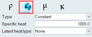
-
Click the Viscosity tab and set the Viscosity value to
1.781e-05.
Figure 17. 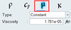
-
Click the Conductivity tab and set the Conductivity
value to 0.02521.
Figure 18. 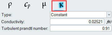
- Close the material creation dialog to return to the Material Library dialog.
-
Select Solid in the Settings menu, click the
My Materials tab, and then click to create a new
solid material model.
-
Name the material Plastic and set the following
values.
The Type should be Constant for each property.
- Density: 1270
- Specific Heat: 1900
- Conductivity: 0.2
- Close the material creation dialog to return to the Material Library dialog.
-
Similarly, create new solid material models named Arnite
and LED with the following properties.
The Type should be Constant for each property.Arnite:
- Density: 1670
- Specific Heat: 2050
- Conductivity: 1.6
LED:- Density: 5500
- Specific Heat: 0.3
- Conductivity: 5.0
Figure 19. 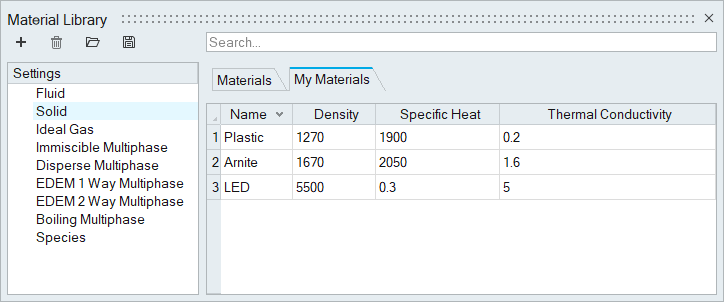
- Close all dialogs and save the model.
Assign Material Properties
-
From the Flow ribbon, click the Material tool.
Figure 20. 
-
Click the lens volume highlighted in the figure below and select
Arnite from the Material drop-down menu.
Figure 21. 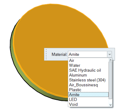
-
On the guide bar, click
 to execute the command and remain in the
tool.
to execute the command and remain in the
tool.
-
Click the housing volume and assign the Plastic material
model.
Figure 22. 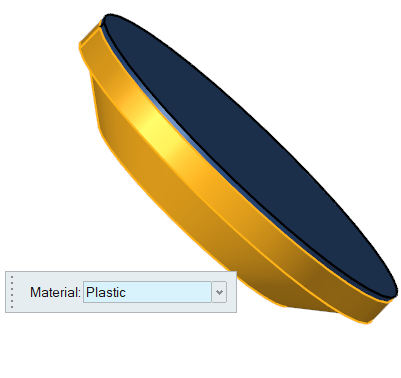
-
On the guide bar, click
to execute the command and remain in the
tool.
- In the Materials legend, right-click Air and select Isolate.
-
Click the air volume and assign the Air_Boussinesq
material model.
Figure 23. 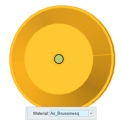
-
On the guide bar, click
to execute the command and remain in the
tool.
- In the Materials legend, right-click Air and select Isolate.
-
Click the bulb volume and assign the LED material
model.
Figure 24. 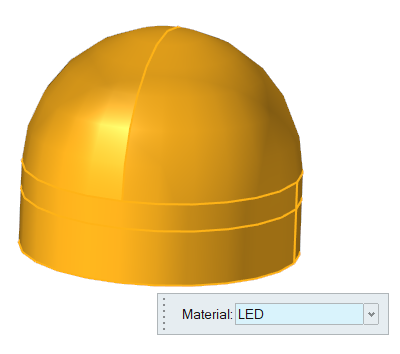
-
On the guide bar, click
 to execute
the command and exit the tool.
to execute
the command and exit the tool.
- Save the model.
Define the Heat Source
-
From the Flow ribbon, click the tool.
Figure 25. 
- In the modeling window, select the bulb volume.
-
In the Heat Source dialog, set the heat source value to
2049180 W/m3.
Figure 26. 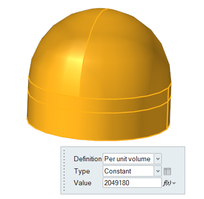
-
On the guide bar, click
to execute
the command and exit the tool.
- Press Esc to exit the Sources tool then press the A key to turn on the display of all solids.
- Save the model.
Define Flow Boundary Conditions
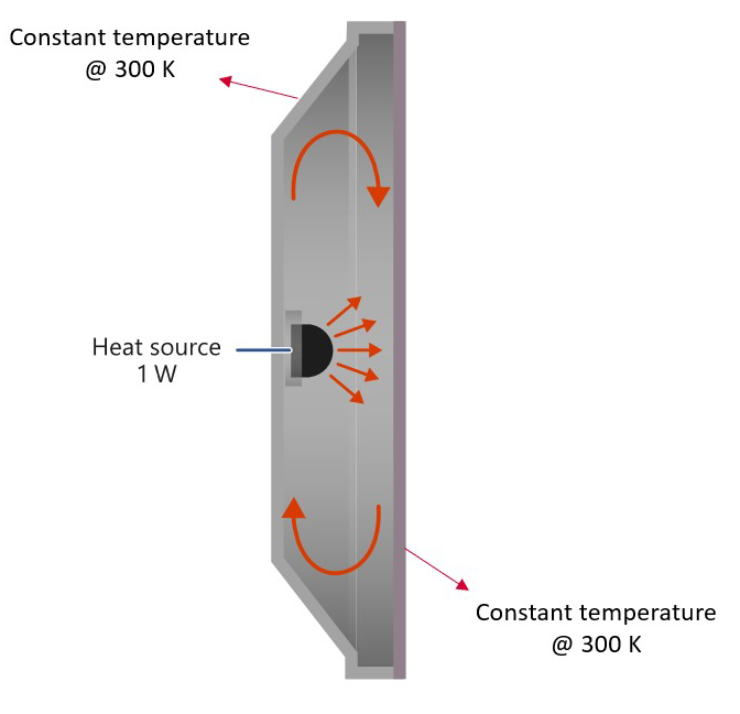
In this problem, all the surfaces are walls and will therefore be assigned the default wall boundary condition. The outer walls of the headlamp will be given a no-slip wall boundary condition with a constant temperature.
-
From the Flow ribbon, click the No Slip tool.
Figure 27. 
-
In the modeling window, select the surfaces highlighted
in the figure below.
Figure 28. 
-
In the microdialog, enter the values shown in the
figure below.
Figure 29. 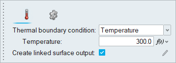
- In the Boundaries legend, double-click Wall, rename it to Outerwalls, and then press Enter.
-
On the guide bar, click
to execute
the command and exit the tool.
- Save the model.
Set Up Radiation
In this step, you will specify the parameters related to the thermal radiation setup.
Define Radiation Model Settings
-
From the Radiation ribbon, Thermal Radiation tools, click the Physics tool.
Figure 30. 
The Radiation Settings dialog opens. - Activate Thermal radiation and set the Radiation model to Discrete Ordinate.
-
Verify that the Radiation quadrature is set to S4.
Figure 31. 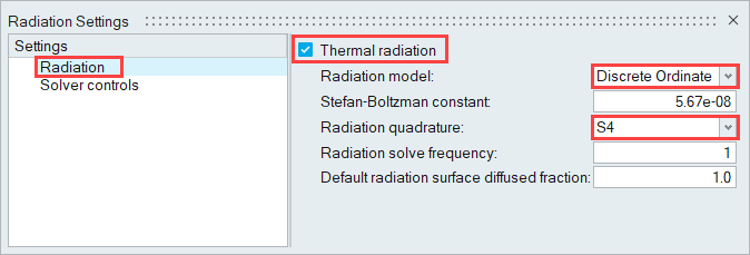
- Close the dialog.
Define the Emissivity Models
-
From the Radiation ribbon, click the
Surface Finish Library
tool.
Figure 32.
The Surface finish library opens.Click to add a
new emissivity model. -
Set the Name of the model to Inner and the Emissivity
value to 0.05 by double-clicking on the entity
fields.
Figure 33. 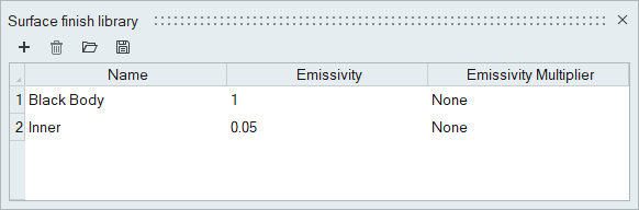
- Close the dialog.
Define the Participating Media Radiation Models
-
From the Radiation ribbon, Participating Media tools, click the Model tool.
Figure 34.
The Participating media model library opens. -
Click to add a
new model.
-
Name the new model Air and assign the following property
values:
- Absorption coefficient - 0
- Scattering coefficient - 0
- Phase coefficient - 0
- Refractive index - 1
-
Similarly, create another model named Lens and assign
the following property values:
- Absorption coefficient - 900
- Scattering coefficient - 0
- Phase coefficient - 0
- Refractive index - 1.57
Figure 35. 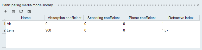
- Close the dialog.
Assign Participating Media Models
-
From the Radiation ribbon, click the
Assign tool.
Figure 36. 
-
Click the lens volume and assign the Lens model from the
microdialog drop-down.
Figure 37. 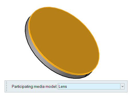
-
On the guide bar, click
to execute the command and remain in the
tool.
- In the Participating Media legend, right-click Lens and select Hide.
-
Select the air volume and assign the Air model.
Figure 38. 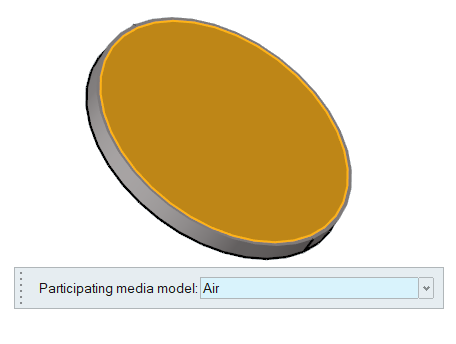
-
On the guide bar, click
to execute the command and remain in the
tool.
- In the Participating Media legend, right-click Air and select Hide.
- Save the model.
Assign Surface Finish Models
-
From the Radiation ribbon, click the
Surface Finish
tool.
Figure 39. 
-
Select only the inner surfaces of the housing - i.e. the housing-air
interface.
Figure 40. 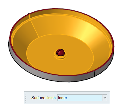
A total of nine surfaces should be selected.
- Assign the Inner model from the microdialog drop-down
-
On the guide bar, click
to execute
the command and exit the tool.
- Turn on the display of all surfaces in the model by pressing the A key.
Define the Radiation Interfaces
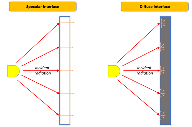
Since the lens and air are defined as semi-transparent media, the interface between the two will be modeled as a specular interface of type: internal. Accordingly, the outer surfaces of the lens will be modeled as external interface radiation surface.
-
From the Radiation ribbon, click the
Interface tool.
Figure 41. 
Notice that all the surfaces except the Lens-Air interface surface are made transparent. Since the Air and Lens volumes are defined as participating media, HyperMesh CFD automatically detects the surfaces that can be defined as an internal radiation interface and only those surfaces will be available for selection when this tool is active. -
Using the box selection method, draw a window around the model.
Observe that the lens-air interface is the only surface that is selected.
-
In the microdialog, set the Radiation diffused fraction
to 0.
Figure 42. 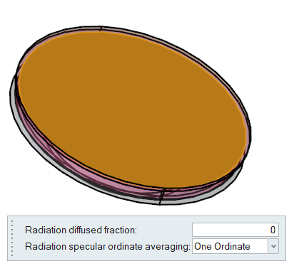
-
On the guide bar, click
to execute
the command and exit the tool.
-
Click the External Boundary tool.
Figure 43. 
- Select the three outer surfaces of the lens volume.
-
In the microdialog, set the Radiation diffused fraction
to 1, the External refractive index to
1, and the External temperature to
300 K.
Figure 44. 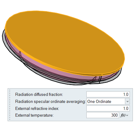
-
On the guide bar, click
to execute
the command and exit the tool.
- Save the model.
Generate the Mesh
In this step, you will define the mesh controls and then generate the mesh.
Define the Surface Mesh Controls
-
From the Mesh ribbon, click the Surface tool.
Figure 45. 
- Using the box selection method, select all the surfaces in the model.
-
In the microdialog, set the Average element size to
0.002.
Figure 46. 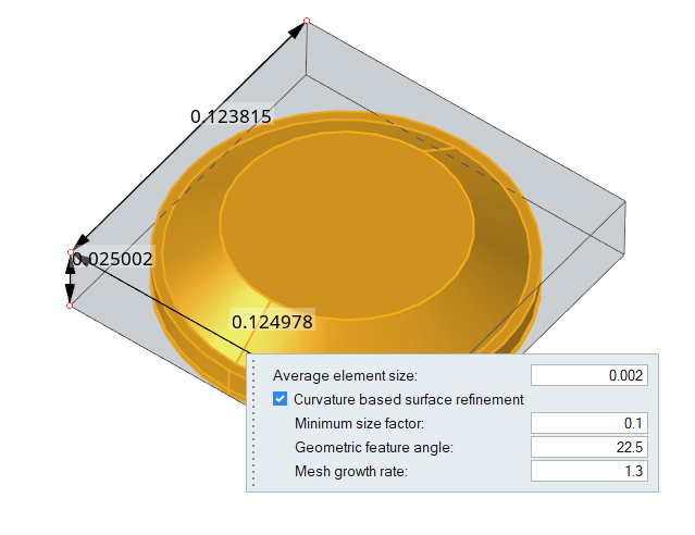
-
On the guide bar, click
to execute the command and remain in the
tool.
-
Select the surface highlighted in the figure below and hide it by pressing the
H key or by right-clicking and selecting
Hide from the context menu.
Figure 47. 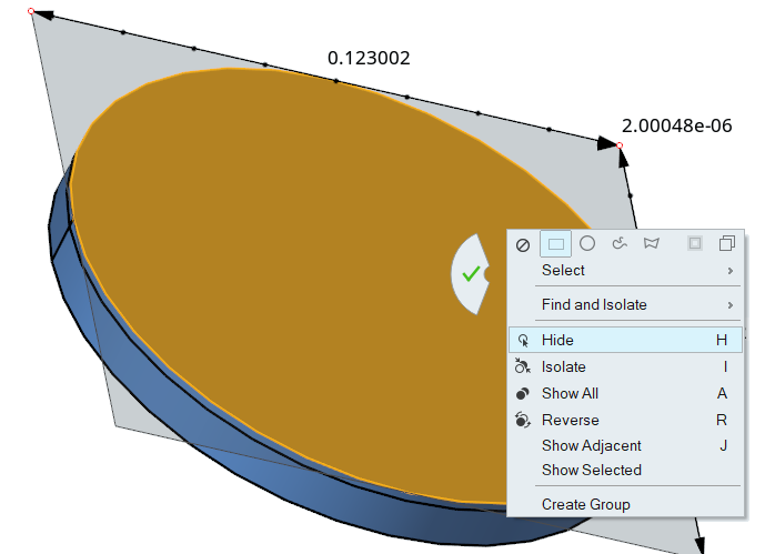
- Select the three surfaces highlighted in the figure below.
-
In the microdialog, set the Average element size to
0.001 and the Mesh growth rate to
1.
Figure 48. 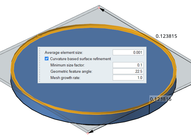
-
On the guide bar, click
to execute
the command and exit the tool.
Define the Boundary Layer Controls
-
From the Mesh ribbon, click the Boundary Layer tool.
Figure 49. 
-
Right-click in the modeling window and go to .
All the fluid wall surfaces should be selected and a microdialog for BL specification appears.
-
Enter the following values in the microdialog:
- First layer thickness definition: Constant
- First layer thickness: 0.0005
- Total number of layers: 4
- Growth method: Constant
- Initial growth rate: 1.3
- Termination policy: Truncate
- Activate the Enable surface mesh modification option
Figure 50. 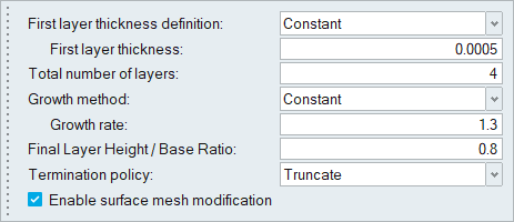
-
On the guide bar, click
to execute
the command and exit the tool.
- Turn on the display of all the surfaces.
Define the Volume Mesh Controls
Since the thickness of the housing and the lens solids are small, you will use the thin layer meshing tool so that when the volume mesh is generated, there will be two layers across the thickness of those solids.
-
From the Mesh ribbon, click the Volume Mesh tool.
Figure 51. 
- Select the housing and the lens solids.
-
In the microdialog,
- Set the Average size to 0.001.
- Set the Growth rate to 1.0.
- Activate the Thin layer meshing option and set the Number of layers to 2.
Figure 52. 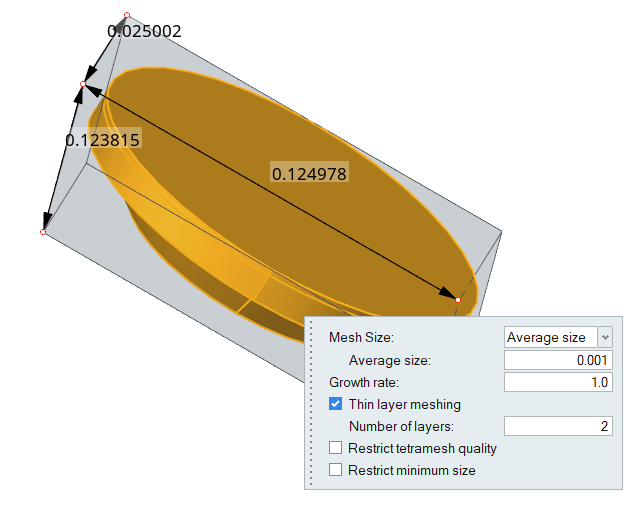
-
On the guide bar, click
to execute
the command and exit the tool.
Generate the Mesh
-
From the Mesh ribbon, click the
Volume tool.
Figure 53. 
The Meshing Operations dialog opens. - Set the Mesh growth rate to 1.
-
Click Mesh.
The Run Status dialog opens. Once the run is complete, the status is updated and you can close the dialog.Tip: Right-click the mesh job and select View log file to view a summary of the meshing process.
- Save the model.
Run AcuSolve
-
From the Solution ribbon, click the Run tool.
Figure 54. 
The Launch AcuSolve dialog opens. - Set the Parallel processing option to Intel MPI.
- Optional: Set the number of processors to 4 or 8 based on availability.
- Expand the Default initial conditions menu and deactivate the Pre-compute flow option.
- Set the x-velocity to 0 and the Temperature to 300.
-
Leave the remaining options as default and click
Run to launch AcuSolve.
Figure 55. 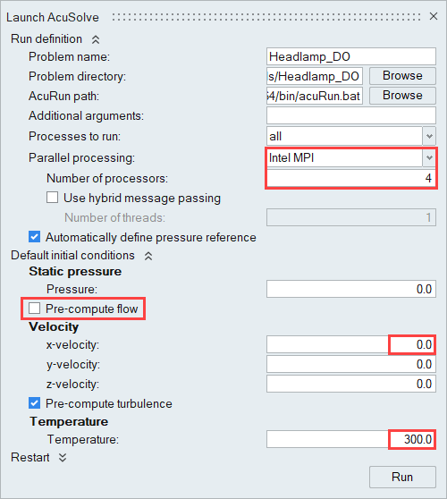
The Run Status dialog opens. Once the run is complete, the status is updated and you can close the dialog.Tip: While AcuSolve is running, right-click the AcuSolve job in the Run Status dialog and select View Log File to monitor the solution process.
Post-Process the Results with HM-CFD Post
- Once the solution is completed, navigate to the Post ribbon.
- From the menu bar, click .
-
Select the AcuSolve
.log file in your problem
directory to load the results for post-processing.
The solid and all the surfaces are loaded in the Post Browser.
-
Click the Slice Planes tool.
Figure 56. 
-
Select the plane perpendicular to the x-axis, as shown in the figure
below.
Figure 57. 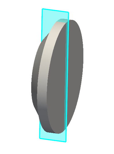
-
Click the Front face on the View Cube to align the
model.
Figure 58. 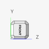
-
Click
 in the slice plane microdialog.
- In the display properties microdialog, set the display to temperature.
-
Activate the Legend toggle and click
 to reset the range.
-
Click
 , set the Legend location to Upper Right
Corner, and the Colormap Name to Rainbow
Uniform.
, set the Legend location to Upper Right
Corner, and the Colormap Name to Rainbow
Uniform.
Figure 59. 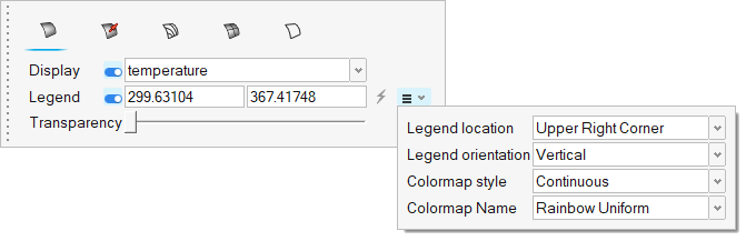
-
Click
 on the guide bar.
-
In the Post Browser, hide the Boundary
Collections.
Figure 60. 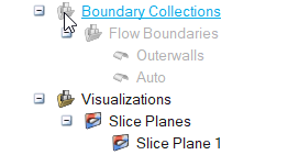
Figure 61. 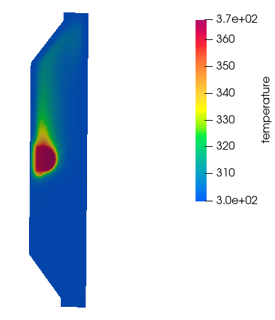
- Right-click Slice Plane 1 in the browser and select Edit.
- Change the display to incident radiation.
-
Click to refresh the legend's range.
-
Click on the guide bar.
Figure 62. 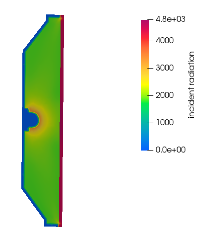
Summary
In this tutorial, you learned how to set up and solve a radiation heat transfer problem in a headlamp using the discrete ordinate radiation model in HyperMesh CFD. You started by importing and cleaning up the geometry and then set up the flow, thermal, and radiation boundary conditions. Once the solution was computed, you processed the results using the Post ribbon where you created contour plots of temperature and incident radiation.