Since version 2026, Flux 3D and Flux PEEC are no longer available.
Please use SimLab to create a new 3D project or to import an existing Flux 3D project.
Please use SimLab to create a new PEEC project (not possible to import an existing Flux PEEC project).
/!\ Documentation updates are in progress – some mentions of 3D may still appear.
Creating an application for machines with step skewing
Introduction
In a Flux Skew project, the type of skewing (i.e., continuous or step) of a machine is a property of the application.
- How to create an application with step skewing.
- Specificities of solid conductor regions
- Example of application.
How to create an application with step skewing
- Only magnetic applications exist in Flux Skew, as discussed in the topic: Flux Skew magnetic applications.
- For all applications in Flux Skew, the Definition tab of the application creation window contains a Skewing definition section. This section must be completed with construction parameters of the skewed machine.
- Skewed mechanical set: in this drop-down menu, the user must choose
between Fixed mechanical set and Rotating mechanical set.
Note: Only the regions linked to the chosen mechanical set will be subjected to skewing. This option allows distinguishing between machines with skewed rotors (usually linked to a rotating mechanical set) or skewed stators (usually linked to a fixed mechanical set).
- Skewing type: in this drop-down menu, the user must choose Step skew.
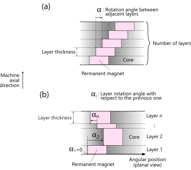
- Topology description: two approaches are available, namely the Simple (homogenous layers) method and the Advanced (layer by layer) method.
- The Simple (homogenous layers) description method is straightforward
and requires only three parameters (accordingly with part (a) of Figure 1):
- the Length unit allowing to choose the unit (or to create a new one) for the Layer thickness;
- the Layer thickness;
- the Rotation angle between adjacent layers, in degrees;
- the Number of layers, or the axial discretization of the
skewed machine after its 3D reconstruction (in post-processing).
Note: This parameter also corresponds to the total number of linked 2D finite element problems solved by Flux Skew along the axial length of the machine during resolution, as discussed in the topic: What is Flux Skew?
- The Advanced (layer by layer) method is also available and allows the
description of more complex topologies (V, W or zig-zag skewing, for
instance). In this approach, the user must fill a table in which each line
represents a skewed layer. Two parameters are required for each layer
(accordingly with part (b) of Figure 1):
- the Length unit allowing to choose the unit (or to create a new one) for the Layer thickness;
- the Layer thickness;
- the Layer rotation angle with respect to the previous one, in degrees.
The remaining tabs of the application creation window are similar to their Flux 2D and Flux 3D counterparts and depend on the specific application chosen by the user.
Once the description of the application is completed, the user is ready to proceed with the 2D description of a rotating electric machine with step skewing in Flux Skew's environment.
Example of application
This example considers the modeling of a step-skewed permanent magnet synchronous machine (PMSM), both in Flux Skew and in Flux 3D.
To compare these modules and the results yielded by them, a three-phase, eight-pole PMSM is considered. Its three-phase winding is distributed between several stator slots, with one phase per slot. Moreover, its rotor (which contains the magnets) is step-skewed: its permanent magnets are distributed into three skewed layers along the axial direction. Each layer has an axial length equal to 125 mm, and the rotation angle between them is 10°.

A simulation representing the same PMSM with step-skewed rotor has been performed in Flux 3D as well.

This behavior is not really surprising, since the Flux 3D project takes into account the flux leakage at the extremities of the machine. This effect is not taken into account in Flux Skew, since it solves a series of linked 2D finite element problems instead, as discussed in the section What is Flux Skew?.
| Flux Skew | Flux 3D | |
|---|---|---|
| Mesh generation time | 30 seconds | 1 hour |
| Solving time | 25 minutes | 11 hours |

It follows from this example that Flux Skew provides results that are in overall good agreement with Flux 3D. This is achieved with a simplified project description and shortened computation times. Even so, the user should always keep in mind the underlying approximations in a Flux Skew simulation, notably while post-processing the results or when comparing them with Flux 3D or with the real device.