Free-shape optimization
Overview
The first version of free-shape optimization has been implemented in Flux 2021.2. Currently, three types of responses to optimize can be chosen in Flux: flux, torque or force. During the optimization, Flux computes the sensitivities of each responses from the adjoint method on the lines to optimize and then launches OptiStruct to run the free-shape optimization process. To run the free-shape optimization, OptiStruct must be installed and the OptiStruct installation path must be set in the FluxSupervisor Options in the Coupled software section. The free-shape optimization moves the mesh nodes of the line you want to optimize to maximize or minimize your responses. This feature will allow the design of new shapes for your devices and will bring better performances.
Available in Beta mode and only in Windows, the free-shape optimization can be run from the Solving menu. Before running an optimization, it is necessary to define the optimization problem (minimization or maximization), the responses (flux, torque or force) the objective function to optimize (a predefined function like avg, maxabs or rms for example or a Compose function defined in an oml file) and the constraints.Example of application
This example may be seen as an extension of the example available in the supervisor in the 2D Application Note section named: Shape Optimization of a synchronous reluctance machine
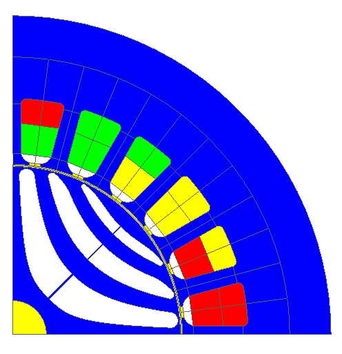
Let's consider the modeling of the following electrical machine represented by only one quarter of the full device.
- Reduce the weight of the rotor
- Increase the mean value of the torque
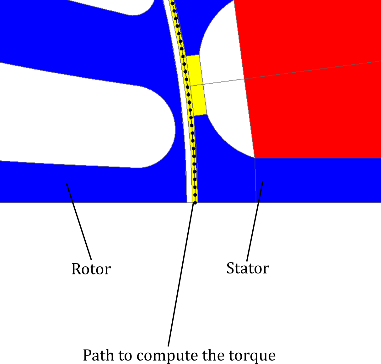
To run the shape optimization, the selected response is the Torque, a path to compute the torque is depicted in the following figure:
- A one axis symmetry constraint
- A constraint on the volume of the rotor in order to decrease its weight
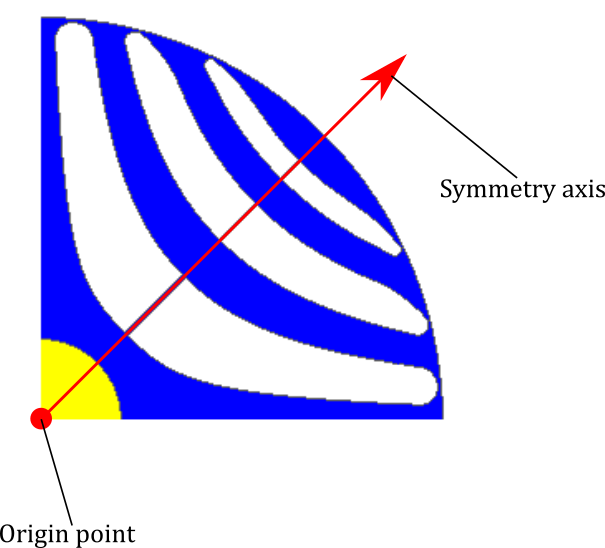
The origin axis is setted to (0,0) and the symmetry axis is setted to (0.5,0.5).
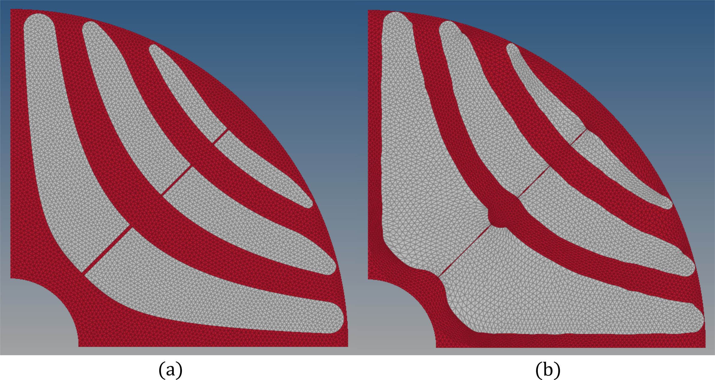
For the constraint on the volume, we want to reduce the volume of iron in the rotor about 20%, in the upper bound the value corresponding to 80% of the total volume is filled, in the lower bound 60% of the volume is filled.
Even if at the starting point the initial design is not between the bounds, the optimization algorithm will deteriorate the objective function in order to find a design that fit the bounds, then the algorithm will start to optimize the design in order to increase or decrease the objective function.
In the objective function, we choose to Maximize the Average of the Torque response previously defined
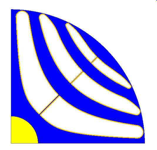
In the end, the lines where the nodes can move are selected as depicted in the figure bellow (the lines are surrounded in yellow):
The scenario is piloted by the mechanical set angle and is covering an electrical period with two degrees per computation step.
| Initial design | Final design | Difference | |
|---|---|---|---|
| Mean torque (N.m) | 11.9 | 12.5 | + 4.8% |
| Rotor weight (kg) | 0.5 | 0.4 | - 20% |