How to parallelize the solving on a single machine

Define the number of cores during solving in the Supervisor

In Flux, the number of cores is defined in the Supervisor as shown below and allows, as seen previously, to perform certain finite element solving tasks in parallel.

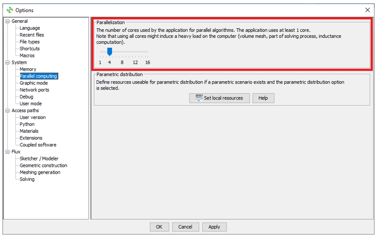
The figure above shows that the number of cores available on the machine is 16 and each instance of Flux will use 4 of them.

It is also important to note that the computation speed according to the number of cores does not decrease linearly, therefore setting this number to the maximum is not necessarily the best choice and may overload the machine. Moreover, when the number of nodes in the project is not large enough, increasing the number of cores will not allow to reduce the computation time.

Available solvers to solve the linear system in Flux

The direct solver is very efficient and requires less memory on small finite element problems like 2D, Skew, or even 3D but with a coarse mesh. However, like any direct solver, when the linear system to solve becomes too large, the memory consumption increases drastically, and the performances in terms of computation time decrease. As soon as the linear system becomes too large, the use of an iterative solver is recommended. The direct solver used by Flux is MUMPS, for more information on this solver, see the MUMPS page.

The parallel iterative solver uses MPI to parallelize large finite element problems with the advantage of significantly reducing memory requirements compared to the direct solver. This solver makes it possible to take advantage of all CPU resources of all computers, laptops, or HPC nodes because of its low memory requirements. The iterative solver used by Flux uses the PETSc library, for more information, see the PETSc page.