Best practices

PERFORMANCE MAPPING – SINE WAVE – MOTOR – EFFICIENCY MAP

Advanced Inputs and their impacts on the test performance

Positioning and objective

General guidelines for a balance between accuracy and computation time

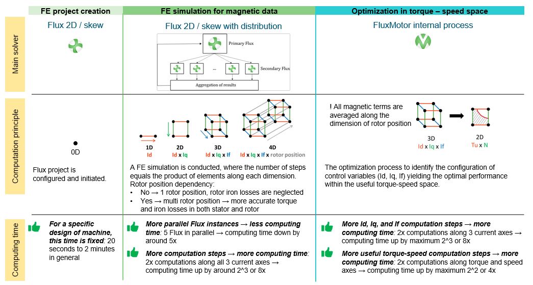
Here below, the process is summarized for a quick understanding of how it is carried out and which factors can influence the overall performance in terms of accuracy and computing time. In general, the machine performance needs to be evaluated within its operational range before looking for optimal configuration of control variables for each torque-speed working point.

Summary of the efficiency map computation process with SMWF as example

1. FE project creation

   In this step, the computing process is set up using inputs and settings provided by the user. The Flux 2D/Skew project is configured and initiated with the appropriate scenario for execution in the subsequent phase. The distribution mode of Flux has no utility at this early stage.

   The only factor impacting the computing time of this step is the design of the machine itself. Factors such as whether it is skewed, the number of poles/slots being simulated, the number of nodes utilized to depict the machine in Flux 2D/Skew, and whether conductors in slots are accounted for in Flux 2D/Skew, all play a role.

   Note: As a general guideline, in the efficiency map, since conductors are not explicitly represented in Flux 2D/Skew, this step typically consumes a relatively short amount of time within the overall computing process, typically ranging from 20 seconds to a minute.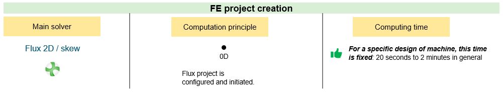

   FE project creation phase of the efficiency map computation process

2. FE simulation for magnetic data

   The Flux 2D/Skew project, previously prepared to analyze the electromagnetic performance of the machine within its defined operational range, is launched.

   It's important to understand that the machine's operational range is determined by the currents supplied to it. For SMPM and RSM machines, this includes the d-axis Jd and q-axis Jq currents, and for SMWF machines, it also includes the excitation current If. During this phase, the supplied current values are varied within their defined ranges to evaluate the machine's electromagnetic performance across all points.

   When the rotor position dependency option is enabled, an additional dimension is introduced to the evaluation of each machine. Consequently:

   • For SMPM and RSM machines: Performance evaluation occurs in a 2-dimensional characteristic space of Jd and Jq when rotor position dependency is disabled, and in a 3-dimensional characteristic space of Jd, Jq, and rotor position when enabled.
   • For SMWF machines: Performance evaluation occurs in a 3-dimensional characteristic space of Jd, Jq, and If when rotor position dependency is disabled, and in a 4-dimensional characteristic space of Jd, Jq, If, and rotor position when enabled.

   Note: Increased level of details in the characteristic space requires more computations, resulting in more detailed performances, as well as longer computing times.

   For example:

   • If the number of computations for Jd and Jq doubles for a test with SMPM, the computation time for this phase may quadruple.
   • Similarly, in the case of SMWF, doubling the number of computations for Jd, Jq, and If can increase computation time by eightfold.
   Additionally, when rotor position dependency is considered, doubling the number of points per electrical period in a test can double the computing time required.

   Note: While rotor position dependency enhances the accuracy of estimating electromagnetic torque and iron losses, it introduces a higher computational cost due to the added dimension in the characteristic space.
   However, this increased cost can be compensated by:

   • Using the half period option for the number of computed electric periods inputs to reduce the number of rotor positions by nearly a half (half of the number of computations per electric periods plus 1 point).
   • Using the distribution mode of Flux, where computing time decreases proportionally with the number of parallel Flux instances employed. For example, running 5 Flux instances concurrently can reduce computing time by up to 5 times.

   Note: The effectiveness of the distribution mode depends on the computer's configuration. For further details regarding distribution mode, performance, and licensing, please refer to the FluxMotor Supervisor document.

   Note: The design of the machine also has a huge impact on the computing time of this step because the more nodes that the FE project uses to describe the machine, the more time and resources are needed to complete the FE simulation.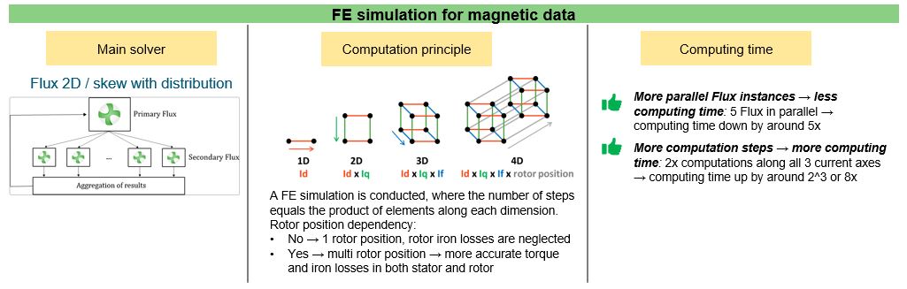

   FE simulation for magnetic data phase of the efficiency map computation process

3. Optimization in torque – speed space
   The machine's performance within its operational range was extensively assessed in the previous step, and the acquired data is utilized in an optimization process to identify optimal control variables. For detailed information on the optimization process, please refer to the section on command modes.

   Note: This optimization step is executed in the backend of FluxMotor, with computing time unaffected by the machine's design. However, two factors can influence the computing time at this stage:

   • The number of computations for Jd, Jq, and If (applicable to SMWF machines): Since the volume of data processed in the optimization process is directly proportional to the number of elements in the machine's characteristic space, doubling the number of elements along each axis (Jd, Jq, and If) can result in an eightfold increase in computing time for SMWF and a fourfold increase for SMPM. For sure, this action brings more accurate data for the optimization process.
   • The number of computations for torque and speed: Increasing the number of computations for these parameters entails optimizing more torque-speed working points. However, since the optimization process at each point begins with values from the closest point, a higher level of detail in the torque-speed space facilitates quicker convergence at each point. While increasing the number of computations for torque and speed generally lengthens computing time in this final step, the relationship is not strictly proportional.

   Note: The choice for the rotor position dependency does not impact the computing time of this step because all electromagnetic data is averaged along the rotor position axis if the rotor position dependency is enabled. The organization of data with or without rotor position dependency is the same for the optimization step. Only the accuracy of the estimation of electromagnetic torque and iron losses are impacted.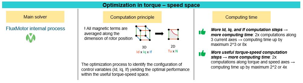

   Optimization in torque – speed space phase of the efficiency map computation process

Examples demonstrating the impact of advanced inputs

However, it's crucial to understand that computing time can vary significantly depending on the setup of the computer used for the analysis. Factors such as hardware specifications, background processes, and system configuration can all impact computing performance and, consequently, computing time.

Therefore, while the results of this benchmark study provide valuable insights into computing time under specific conditions, users should be aware that actual computing times may differ based on their individual computer setups.

1. Accuracy versus computing time in case of a SMPM

   In this example, the efficiency map of a SMPM is analyzed under various configurations of input parameters along the current axis (Jd, Jq) and rotor position axis within the characteristic space. The goal is to illustrate how these input configurations influence the accuracy and computational time of the efficiency test.

   Let's consider a SMPM with the following specifications:

   • 8 poles
   • 48 slots
   • 4000 nodes represented in the FE project of Flux 2D.

   In this instance, the distribution mode of Flux is activated with 5 Flux instances running in parallel.

   Additionally, for computations involving rotor position dependency, the half period computation mode is selected.

   And for the final torque – speed space, each axis is discretized by 30 elements so that the interpolation used for the comparison process can be evaluated with the most accurate.

   Six test configurations are compared, each denoted by the rule: MSX-Y-Z-W, where:

   • X indicates the presence of rotor position dependency (1 for No, 2 for Yes).
   • Y represents the number of computations along the Jd axis.
   • Z represents the number of computations along the Jq axis (Y equals Z).
   • W denotes the number of rotor positions (W equals 1 if X equals 1 or if there is no rotor position dependency).
   The six configurations are as follows:

   • MS2-10-10-100: This serves as the reference for comparison, offering high-resolution data in the characteristic space, ensuring highly reliable computation of iron losses, total losses, and efficiency
   • MS2-10-10-40: To observe the impact of reducing the number of rotor positions.
   • MS2-6-6-40: To observe the impact of reducing elements along the current axis.
   • MS2-6-6-30 and MS2-6-6-20: To explore the effect of decreasing the number of rotor positions to its lower limit.
   • MS1-6-6-1: To observe the impact of neglecting rotor position dependency.
   Each model is compared to the reference model, analyzing efficiency, total losses, and iron losses within the map according to the following criteria:

   • Efficiency: Deviation calculated as the absolute difference between the efficiency percentages of the actual and reference models.
   • Total losses: Deviation calculated as the absolute difference between the total losses of the actual and reference models, divided by the total losses of the reference model, and expressed as a percentage.
   • Iron losses: Deviation calculated as the absolute difference between the iron losses of the actual and reference models, divided by the iron losses of the reference model, and expressed as a percentage.

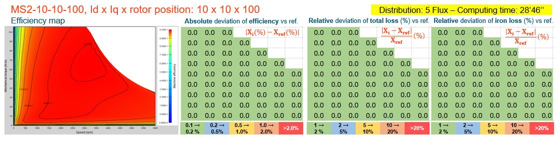
   Example of SMWF efficiency tests – Reference model with 10 steps for current and 100 rotor positions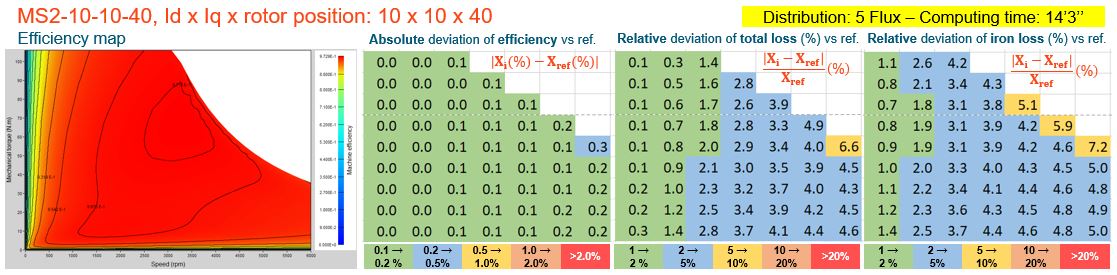

   Example of SMWF efficiency tests – Reference model with 10 steps for current and 40 rotor positions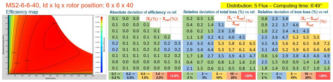

   Example of SMWF efficiency tests – Reference model with 6 steps for current and 40 rotor positions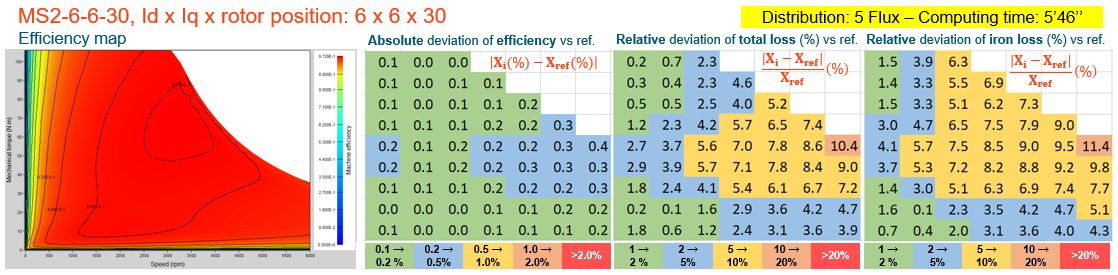

   Example of SMWF efficiency tests – Reference model with 6 steps for current and 30 rotor positions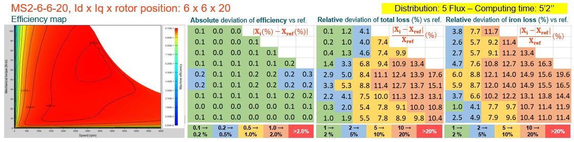

   Example of SMWF efficiency tests – Reference model with 6 steps for current and 20 rotor positions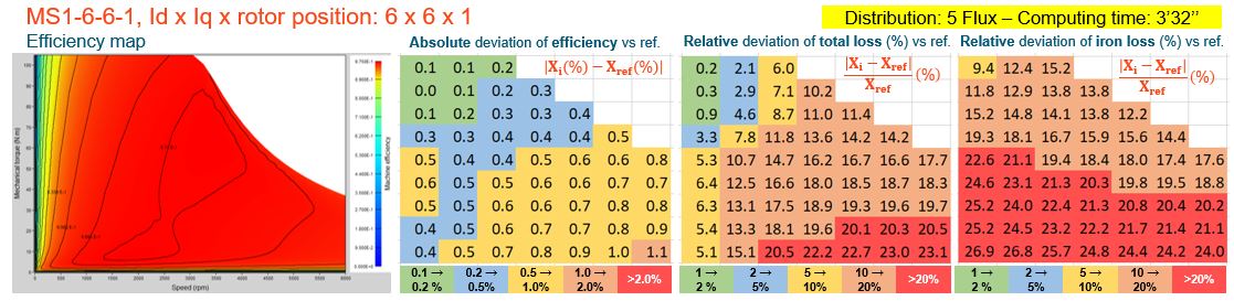

   Example of SMWF efficiency tests – Reference model with 6 steps for current and 1 rotor position (without rotor position dependency)

   Observations:

   • Computation times range from 3 minutes to approximately 30 minutes, progressively decreasing from the first to the sixth configuration as the number of computations decreases.
   • All models yield nearly identical efficiency maps, with deviations consistently minimal (less than 1% of efficiency) as evident in the second figure of each model. However, deviations increase from configuration 2 to 6 due to reductions in elements along current axes and the number of rotor positions.
   • Closer examination of total losses and iron losses reveals the impact of the number of rotor positions considered in the computation. Fewer positions lead to greater deviation compared to the reference. For instance, with only 20 positions, iron losses deviation can reach up to 20% in most areas, whereas with 40 positions, accuracy improves significantly.
   • Utilizing six elements along current axes and 40 rotor positions appears to reach a balance between accuracy and computation time.
   • Models without rotor position dependency exhibit poor estimations of iron losses in this particular machine. However, if only the efficiency map is of concern, this limitation may be acceptable.
2. Recommended inputs for SMPM and RSM with distribution mode disabled
   Below is an example for SMPM. Let's consider a SMPM with the following specifications:

   • 8 poles
   • 48 slots
   • 4000 nodes represented in the FE project of Flux 2D.

   In this instance, the distribution mode of Flux is deactivated, so only 1 Flux instance is run.

   Additionally, for computations involving rotor position dependency, the half period computation mode is selected.

   Thus, the number of rotor positions per electric period varies as follows:

   • For 21, 7, or 26 rotor positions, there are respectively 40, 13, and 50 positions per electric period.
   For each configuration of rotor position dependency (Yes/No), three sets of inputs are provided, each with different priorities for accuracy and computing time:

   • The recommended setting offers highly accurate results within an acceptable computing time, taking up to 2 minutes without rotor position dependency and 20 minutes with it.
   • The basic setting provides preliminary results indicating performance trends with acceptable accuracy in the shortest computing time, taking up to 2 minutes without rotor position dependency and 8 minutes with it.
   • The advanced setting delivers very accurate results but requires significant computing time, taking up to 5 minutes without rotor position dependency and 75 minutes with it. Memory issues may arise as finer characteristic space requires more memory resources. Refer to FluxMotor Supervisor help for guide on how to setup memory configuration of FluxMotor.

   Note: As a general guideline, it's recommended to perform 6 computations along each current axis and have 40 rotor positions per electric period when the rotor position dependency mode is enabled. With the half period computation mode, only 21 points are computed.

   Note: See the next example to understand the power of distribution mode in reducing computing time.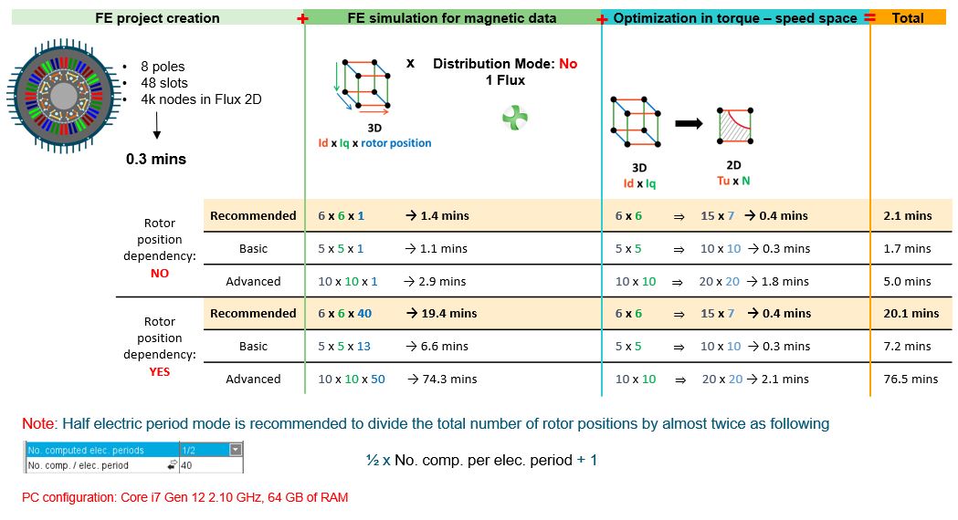

   Recommended inputs for SMPM efficiency map tests with distribution mode disabled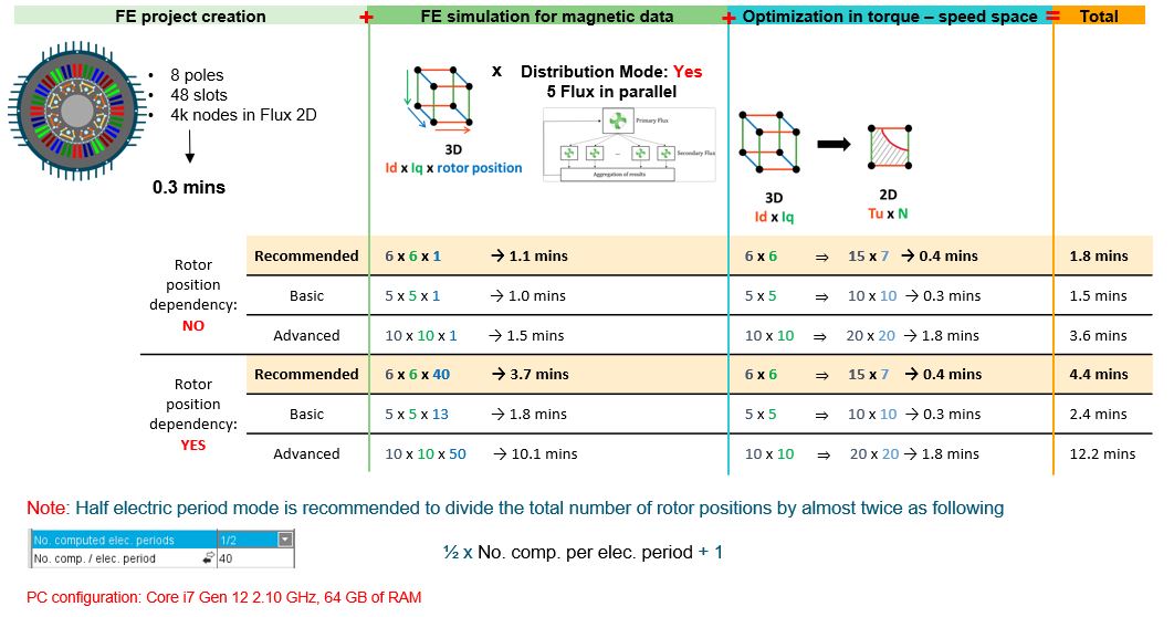

   Recommended inputs for SMPM efficiency map tests with distribution mode enabled

3. Recommended inputs for SMPM and RSM with distribution mode enabled
   Below is an example for SMPM. Let's consider a SMPM with the following specifications:

   • 8 poles
   • 48 slots
   • 4000 nodes represented in the FE project of Flux 2D.

   In this instance, the distribution mode of Flux is activated with 5 Flux instances running in parallel.

   Additionally, for computations involving rotor position dependency, the half period computation mode is selected.

   Thus, the number of rotor positions per electric period varies as follows:

   • For 21, 7, or 26 rotor positions, there are respectively 40, 13, and 50 positions per electric period.
   And because the SMWF benefits from the advantages of both the SMPM and RSM, the 1st and 2nd quadrants are selected in the backend for the FE simulation step. Therefore, the number of steps for Id varies as follows:

   • For 11, 9, or 19 Id values, there are respectively 6, 5, and 10 Id values per quadrant.
   For each configuration of rotor position dependency (Yes/No), three sets of inputs are provided, each with different priorities for accuracy and computing time:

   • The recommended setting offers highly accurate results within an acceptable computing time, taking up to 2 minutes without rotor position dependency and 5 minutes with it.
   • The basic setting provides preliminary results indicating performance trends with acceptable accuracy in the shortest computing time, taking up to 1.5 minutes without rotor position dependency and 3 minutes with it.
   • The advanced setting delivers very accurate results but requires significant computing time, taking up to 4 minutes without rotor position dependency and 15 minutes with it. Memory issues may arise as finer characteristic space requires more memory resources. Refer to FluxMotor Supervisor help for guide on how to setup memory configuration of FluxMotor.

   Note: As a general guideline, it's recommended to perform 6 computations along each current axis and have 40 rotor positions per electric period when the rotor position dependency mode is enabled. With the half period computation mode, only 21 points are computed.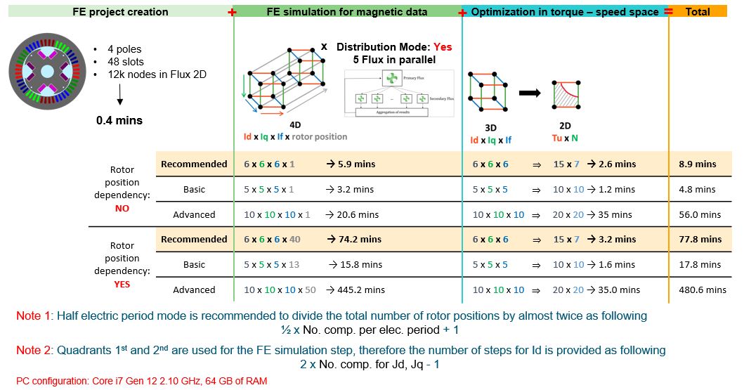

   Recommended inputs for SMWF efficiency map tests with distribution mode enabled