Delay Process
This option allows the user to visualize the Delay Process, that is, a visualization of the signal emitted by the ultrasound sources in the time domain, as it is received at an observation point. When the user selects this option, the following panel is shown:
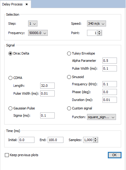
In this panel, the user needs to select the step, frequency, observation point and speed of sound they want to show the results for. In addition, the user needs to select one of the multiple signal shapes:
- Dirac Delta A instantaneous pulse.
- CDMA A random distribution of pulses centred with positive (high) a negative (low) levels. Note that a low or high level is considered as a Pulse. The "Length" parameter determines the number of pulses to be generated, while "Pulse Width" refers to the time duration of each pulse, in milliseconds.
- Sinusoid A sinusoidal signal. The "Frequency" is the frequency of the sinusoidal signal, in kHz. The "Phase" is the initial phase of the sinusoidal signal, in degrees. The "Duration" is the total length of the generated sinusoid in the time domain, in milliseconds.
- Tukey Envelope A Gaussian signal enveloped by a rectangular pulse. The "Alpha Parameter" defines the slope of the Gaussian curve. The higher is this parameter, the more enveloped by the rectangular pulse is the generated signal. The "Pulse Width" defines the total length of the generated signal in the time domain, in milliseconds.
- Gaussian pulse A Gaussian pulse defined by its sigma parameter, in milliseconds.
- Custom signal A user-defined signal (by a user function). In this drop-down list, only functions that return a double value and accept no arguments will be shown. The user function defines the base signal function, that must be centered at t=0. This function is then multiplied by the field value of each ray, translated in time by the propagation of the ray and finally the value of all functions are added at each point to obtain the Delay Process plot.
The following is the example of a user-function that can be used as a custom signal (a square signal of amplitude 1 and 3ms long):
double square_signal(){
 double tms = $t * 1000.0;
 double DURATION_MS = 3;
 if (tms <= -DURATION_MS/2 || tms >= DURATION_MS/2) {
  return 0.0;
 } else {
  return 1.0;
 }
}
The function used as a custom signal has access to three special variables, prefixed by the dollar symbol:
- $t The time value, in seconds, the function is sampled at.
- $freq The selected frequency, in Hz.
- $sound_speed The selected speed of sound, in m/s.
Additionally, the "Time (ms)" panel allows the user to specify the time interval they want to see the results for. The "Initial" and "Final" fields represent the bounds of the time interval, while the "Samples" field is the number of evenly-spaced points that will be calculated within the time interval and therefore the number of points of the generated plot.
The "Keep previous plots" option allows the user to choose whether they want to preserve the previously plotted graphs (which could be useful if the user wants to compare several plots) or they want to clear all previous plots. This option only has an effect for signals different than "Dirac Delta" (which are always shown in a different panel each time).
When the user has finished setting the parameters, they need to click on the "OK" button to plot the Delay Process results.
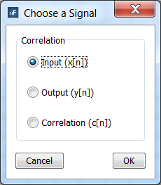
Only when the CDMA signal has been selected, the window represented below asks the selection of the Correlation Signal to be plotted with the following options.
- Input (x[n]) the original CDMA signal is represented.
- Output (y[n]) the received CDMA signal is represented
- Correlation (c[n]) the correlation on the received signal is represented.
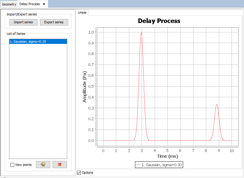
In the plot viewer, the user can delete or change the color of the displayed series, as well as import or export series from/to text files.