View Porosity Analysis Results

Use to view the results of a porosity analysis. You can view shrinkage percentage, temperature evolution, solid fraction, and solidification times for a selected run and load case.

1. Click the Show Porosity Analysis Results tool on the Porosity icon.
   
   The Analysis Explorer opens.
   
   
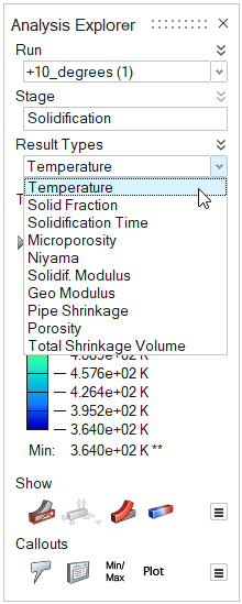
2. Porosity analysis produces four different result types for each load case. Click on a Result Type to view the results.
   • Temperature is a plot of the changes in temperature during the solidification process.
   • Solid Fraction displays the solidification pattern. Drag the arrow to change the solid fraction value, which ranges from 0 to 1. For example, if the animation is set to 0.7 (in most cases, this corresponds to the value at which the liquid stops flowing), the solidified material (above 0.7) will be shown as transparent, while liquid material (below 0.7) is shown in yellow.
   • Solidification Time uses a colored legend to show the time required to fill different areas within the part. This helps you identify which areas will fill first and predict possible areas of cold welding.
   • Microporosity is based on the Dimensionless Niyama criterion. This method avoids the need to know the threshold Niyama value below which shrinkage porosity forms; such threshold values are generally unknown and alloy dependent. The dimensionless criterion accounts for both the local thermal conditions (as in the original Niyama criterion), but also considers more things like pressures, material properties, and parameter properties.
   • Niyama is commonly used by foundries to detect solidification shrinkage defects. It is defined as the local thermal gradient divided by the square root of the local cooling rate. Low temperature gradients cause the material to have less pressure to fill the interdendritic spaces and a high cooling rate, thus it solidifies faster and the material has less time to fill the interdentric spaces. The lower the value, the higher the probability of shrinkage.
   • Solidification Modulus is used to set a proper feeding system by adjusting the modulus of the risers. This calculation is based on the modulus (the ratio of the casting volume to the surface area) and solidification time (Chorinov's rule).
   • Geometric Analysis is an alternative method for calculating the modulus, which is used to set a proper feeding system by adjusting the modulus of the risers. This calculation is based on geometric and solidification data where data image processing is used to post-process the results.
   • Pipe Shrinkage is similar to shrinkage porosity (mass deficit produced by the metal contraction), but it occurs when the top surface is open to the atmosphere. Therefore, as the shrinkage cavity forms, air compensates.
   • Porosity shows areas where the ratio of voids to solid areas is greater than or equal to the specified percentage value. This is the macro porosity or shrinkage porosity.

     Click the legend to change the percentage value.

   • Total Shrinkage Volume is the combination of Pipe Shrinkage and Porosity results and provides the volume of the total amount of macro porosity.
3. Use the scalable results slider to provide a color gradient for the selected result type.

   
   
   

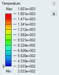
   • To change the upper or lower bound for the results slider, click on the bound and enter a new value. Click the reset button to restore the default values.
   • To filter the results so that areas on the model with results greater than a specified value are masked, click and drag the arrow on the results slider.
   • To change the legend color for the result type, click the icon next to the results slider and select Legend Colors.
4. Use the icons under Show to determine what is made visible in the modeling window for the analysis.
   • Show/hide the initial shape as a reference.
   • Show/hide loads and supports. You can also show only the current loads and supports.
   • Show/hide the deformed shape as a reference.
   • Show/hide contours. Click the icon to reveal additional options related to contours. Select Interpolate during animation to animate the result contour. Select Blended contours to toggle between blended and nonblended contours.