Finite Element Formulation
Finite Element Approximation
- Interpolating shape functions
- Position vector of node
It is worth pointing out that the velocity is a material time derivative of displacements, that is, the partial derivative with respect to time with the material coordinate fixed.
Emphasis is placed on the fact that shapes functions are functions of the material coordinates whatever the updated or the total Lagrangian formulation is used. All the dependency in the finite element approximation of the motion is taken into account in the values of the nodal variables.
Where, are the virtual nodal velocities.
with the part of the boundary where traction loads are imposed.
Internal and External Nodal Forces
As in Virtual Power Term Names, you define the nodal forces corresponding to each term in the virtual power equation.
These nodal forces are called internal because they represent the stresses in the body. The expression applies to both the complete mesh or to any element. It is pointed out that derivatives are taken with respect to spatial coordinates and that integration is taken over the current deformed configuration.
Mass Matrix and Inertial Forces
Discrete Equations
Equation of Motion for Translational Velocities
Equation of Motion for Angular Velocities
- Principal moments of inertia about the x, y and z axes respectively
- Angular accelerations expressed in the principal reference frame
- Angular velocities
- Principal externally applied moments
- Principal internal moments
The vector function is computed for a value of at . Equation 30 is used for rigid body motion.
- Diagonal inertia matrix
- Externally applied moment vector
- Internal moment vector
- Anti-hourglass shell moment vector
Element Coordinates
Finite elements are usually developed with shape functions expressed in terms of an intrinsic coordinates system . It is shown hereafter that expressing the shape functions in terms of intrinsic coordinates is equivalent to using material coordinates.
- The domain in the intrinsic coordinates system
- The current element domain
- The initial reference element domain
is associated with the direction .
is associated with the direction .
is associated with the direction .
- The map from the intrinsic coordinates system to the initial configuration:
(32) - The map from the intrinsic coordinates system to the current configuration:
(33) - The map from the initial to the current configuration:
(34)
Isoparametric elements use the same shape functions for the interpolation of and .
Integration and Nodal Forces
In practice, integrals over the current domain in the definition of the internal nodal forces (Equation of Motion for Translational Velocities, Equation 25), of the external nodal forces (Equation of Motion for Translational Velocities, Equation 24) and of the mass matrix have to be transformed into integrals over the domain in the intrinsic coordinate system .
- The Jacobian determinant of the transformation between the current and the initial configuration
- The Jacobian determinant of the transformation between the current configuration and the domain in the intrinsic coordinate system
- The Jacobian determinant of the transformation between the reference configuration and the intrinsic coordinate system
and obtained from Equation 42.
External forces and the mass matrix can similarly be integrated over the domain in the intrinsic coordinate system.
Function Derivatives
Usually, it is not possible to have closed form expression of the Jacobian matrix. As a result the inversion will be performed numerically and numerical quadrature will be necessary for the evaluation of nodal forces.
Numerical Quadrature: Reduced Integration
- Number of integration points in the element
- Eeight associated to the integration point
For full integration, the number of integration points is sufficient for the exact integration of the virtual work expression. The full integration scheme is often used in programs for static or dynamic problems with implicit time integration. It presents no problem for stability, but sometimes involves locking and the computation is often expensive.
Reduced integration can also be used. In this case, the number of integration points is sufficient for the exact integration of the contributions of the strain field that are one order less than the order of the shape functions. The incomplete higher order contributions to the strain field present in these elements are not integrated.
The reduced integration scheme, especially with one-point quadrature is widely used in programs with explicit time integration to compute the force vectors. It drastically decreases the computation time, and is very competitive if the spurious singular modes (often called hourglass modes which result from the reduced integration scheme) are properly stabilized. In two dimensions, a one point integration scheme will be almost four times less expensive than a four point integration scheme. The savings are even greater in three dimensions. The use of one integration point is recommended to save CPU time, but also to avoid "locking" problems, for example, shear locking or volume locking.
Shear locking is related to bending behavior. In the stress analysis of relatively thin members subjected to bending, the strain variation through the thickness must be at least linear, so constant strain first order elements are not well suited to represent this variation, leading to shear locking. Fully integrated first-order isoparametric elements (tetrahedron) also suffer from shear locking in the geometries where they cannot provide the pure bending solution because they must shear at the numerical integration points to represent the bending kinematic behavior. This shearing then locks the element, that is, the response is far too stiff.
On the other hand, most fully integrated solid elements are unsuitable for the analysis of approximately incompressible material behavior (volume locking). The reason for this is that the material behavior forces the material to deform approximately without volume changes. Fully-integrated solid elements, and in particular low-order elements do not allow such deformations. This is another reason for using selectively reduced integration. Reduced integration is used for volume strain and full integration is used for the deviatoric strains.
However, as mentioned above, the disadvantage of reduced integration is that the element can admit deformation modes that are not causing stresses at the integration points. These zero-energy modes make the element rank-deficient which causes a phenomenon called hour-glassing; the zero-energy modes start propagating through the mesh, leading to inaccurate solutions. This problem is particularly severe in first-order quadrilaterals and hexahedra.
Zero-energy or hourglass modes are controlled using a perturbation stabilization as described by Flanagan-Belytschko 1, or physical stabilization as described in 2 (Element Library).
So, for isoparametric elements, reduced integration allows simple and cost effective computation of the volume integrals, in particular on vectorized supercomputers, and furnishes a simple way to cope with locking aspects, but at the cost of allowing hour-glassing.
Numerical Procedures
- For the displacement, velocity and acceleration at a particular time step, the external force vector is constructed and applied.
- A loop over element is performed, in which the internal and hourglass forces are
computed, along with the size of the next time step. The procedure for this loop is:
- The Jacobian matrix is used to relate displacements in the intrinsic coordinates
system to the physical space:
(51) - The strain rate is calculated:
(52) - The stress rate is calculated:
(53) - Cauchy stresses are computed using explicit time integration:
(54) - The internal and hourglass force vectors are computed.
- The next time step size is computed, using element or nodal time step methods (Dynamic Analysis)
- The Jacobian matrix is used to relate displacements in the intrinsic coordinates
system to the physical space:
- After the internal and hourglass forces are calculated for each element, the algorithm proceeds by computing the contact forces between any interfaces.
- With all forces known, the new accelerations are calculated using the mass matrix and
the external and internal force vectors:
(55) - Finally, time integration of velocity and displacement is performed using the new
value.
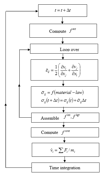
Figure 1. Numerical Procedure