
OS-E: 6005 Modal Complex Eigenvalue Analysis
This example demonstrates the Rotor Dynamics with modal complex eigenvalue analysis using two coaxial rotors in OptiStruct.
Model Files
Model Description
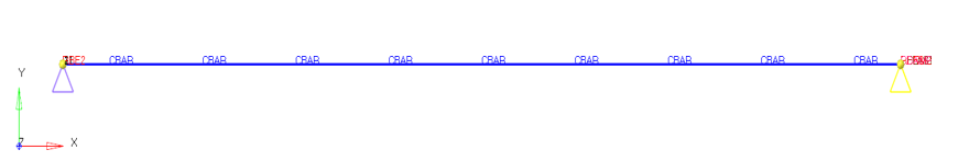
This example consists of two coaxial rotors modeled using 1D elements (CBAR). One end of each rotor is constrained, and this end is attached to the stator using rigid elements as per convention. The constrained nodes represent the ends of the stator. Spring (CELAS) and damper (CDAMP) elements are used to model the bearings at the rotor-stator junction.
Relative spin between the two rotors is also defined. Synchronous and asynchronous analyses are performed at different maximum rotor speeds. The complex modes of the structure are extracted to determine the critical frequencies and the Campbell diagram is generated.
CONM2 elements are attached to the rotor. PARAM, GYRO1D, NO are defined in the model to ignore the contribution from 1D elements in the gyroscopic matrix calculation and only consider the CONM2 elements. The mass properties for the CONM2 element are defined with respect to a user-defined rectangular coordinate system.
The Campbell diagram is used to plot the modes from the asynchronous analysis and identify the critical speed. NC2O mode tracking method is used.
| FE Model | 1D Elements |
|
| Material | Material MAT1 | Rotor (MAT1):
|
| Reference Guide Entries | Keywords | RGYRO, ROTORG, RSPINR, DDVAL, RFORCE, RSPEED, EIGC, EIGRL |
Results
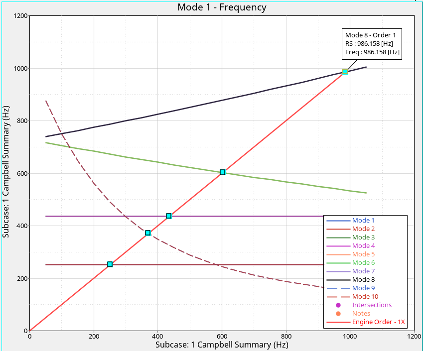
The .out file is used to plot the Campbell diagram in HyperGraph 2D. Refer to Rotor Dynamics for more details. An engine order of 1 is used and this plots a line of unit slope. Modes which intersect this line satisfy the condition that Rotor Speed = Whirl Frequency.
From the Figure 2, 5 intersections have been identified. The critical speed occurs for the first forward whirl mode (forward whirl modes have positive slope) that intersects the line of 1st engine order. Based on the graph, the critical speed occurs for the 8th mode with a frequency of 986.158 Hz. Other modes which intersect are either linear (flat lines) resonant frequency modes or backward whirl (negative slope), which are not of significance.
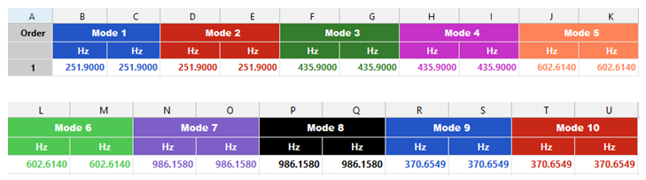
The second subcase corresponds to synchronous analysis and these modes match the intersection points in the Campbell diagram obtained from asynchronous analysis.
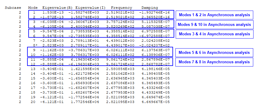
In this way, the critical speed is identified from the Campbell diagram and the modes from asynchronous and synchronous analysis are shown to be very close to each other.