OS-T: 3030 Random Response Optimization
In this tutorial you will perform a topography optimization with random response on a flat plate.
Launch HyperMesh and Set the OptiStruct User Profile
-
Launch HyperMesh.
The User Profile dialog opens.
-
Select OptiStruct and click
OK.
This loads the user profile. It includes the appropriate template, macro menu, and import reader, paring down the functionality of HyperMesh to what is relevant for generating models for OptiStruct.
Import the Model
-
Click .
An Import tab is added to your tab menu.
- For the File type, select OptiStruct.
-
Select the Files icon
 .
A Select OptiStruct file browser opens.
.
A Select OptiStruct file browser opens. - Select the panel.fem file you saved to your working directory.
- Click Open.
- Click Import, then click Close to close the Import tab.
Set Up the Optimization
Define Topography Design Variables
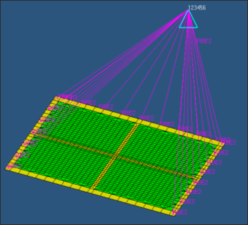
For a topography optimization, a design space and a bead definition need to be defined.
In this step, the design space is composed of the shell elements with the property PSHELL_5. A minimum bead width of 0.4, a bead height of 1, and draw angle of 60 degrees is used in the bead definition. A 2-plane symmetrical pattern grouping constraint is defined to generate a symmetrical bead design.
- From the Analysis page, click the optimization panel.
- Click the topography panel.
-
Create a topography design space definition.
- Select the create subpanel.
- In the desvar= field, enter plate.
- Using the props selector, select PSHELL_5.
- Click create.
A topography design space definition, plate, has been created. All elements organized into the PSHELL_5 component collector(s) are now included in the design space. -
Create a bead definition for the design space plate.
A bead definition has been created for the design space plate. Based on this information, OptiStruct will automatically generate bead variable definitions throughout the design variable domain.
-
Adding pattern grouping constraints.
-
Set the anchor node, first node, and second node selectors to
coordinates, then enter the values indicated
in Figure 2 to define a 2-plane symmetry
constraint.
Figure 2. 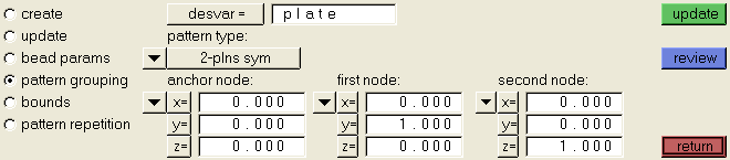
-
Set the anchor node, first node, and second node selectors to
coordinates, then enter the values indicated
in Figure 2 to define a 2-plane symmetry
constraint.
-
Update the bounds of the design variable.
The upper bound sets the upper bound on grid movement equal to UB*HGT and the lower bound sets the lower bound on grid movement equal to LB*HGT.
- Click return to go to the Optimization panel.
Create Design Response for Random Response Optimization
- Click the responses panel.
- In the response = field, enter psdaccl.
- Set the response type to psd acceleration.
-
Click , then enter 67 in the id= field.
Node 67 is close to the center of the plate.
- Select dof1 for the PSD acceleration in X direction.
-
Click randps= and select
RANDPS100.
This specifies the Power Spectral Density for the random response analysis.
- Leave frequencys set to all freq.
- Set the region to no regionid.
- Click create.
- Click return to go back to Optimization Setup panel.
Define the Objective Reference
- From the Analysis page, Optimization panel, click the obj reference panel.
- In the dobjref= field, enter psdacclref.
-
Select pos reference, and enter 1.0e6.
The values of the response, psdaccl, will be normalized by the negative and positive reference values.
- Select neg reference, and enter -1.0.
- Click response and select psdaccl.
-
Set the loadsteps selection option to all.
This ensures the DOBJREF entry is applied to all subcases.
- Click create.
- Click return to go back to the Optimization panel.
Define the Objective Function
- Click the objective panel.
- Verify that minmax is selected.
- Click dobjrefs and select psdacclref.
- Click create.
- Click return twice to exit the Optimization panel.
Run the Optimization
- From the Analysis page, click OptiStruct.
- Click save as.
-
In the Save As dialog, specify location to write the
OptiStruct model file and enter
panel_complete for filename.
For OptiStruct input decks, .fem is the recommended extension.
-
Click Save.
The input file field displays the filename and location specified in the Save As dialog.
- Set the export options toggle to all.
- Set the run options toggle to optimization.
- Set the memory options toggle to memory default.
-
Click OptiStruct to run the optimization.
The following message appears in the window at the completion of the job:
OPTIMIZATION HAS CONVERGED.
FEASIBLE DESIGN (ALL CONSTRAINTS SATISFIED).
OptiStruct also reports error messages if any exist. The file panel_complete.out can be opened in a text editor to find details regarding any errors. This file is written to the same directory as the .fem file. - Click Close.
View the Results
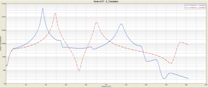
HyperView is used to view the bead design generated from the topography optimization. “XYPUNCH, ACCE, PSDF/67(T1RM)” was used to output the PSD accelerations to punch files. The PSD plot from punch output can be viewed with HyperGraph. The RMS and peak PSD values are output to the .peak file and can be viewed with text editor.
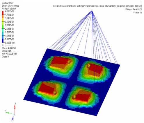
View the Bead Patterns
-
From the OptiStruct panel, click HyperView.
HyperView is launched and the optimization results (_des.h3d) are loaded.
-
On the Results toolbar, click
 to open the Contour panel.
- Set the Result type to Shape Change (v).
- In the Results Browser, select the last iteration.
- In the Contour panel, click Apply.
View the PSD Results
- Launch HyperGraph.
-
On the Curves toolbar, click
 to
open the Build Plots panel.
to
open the Build Plots panel.
- Load the panel_complete.pch file.
- Set the X Type to Frequency (Hz).
-
Set Group 1 Acceleration to Y Type.
Node id 67 and X_Translation are highlighted.
-
Click Apply.
The PSD plot of acceleration in X direction on node 67 at iteration 0 is loaded.
-
On the Annotations toolbar, click
 to
open the Axes panel and convert the linear plot of PSD acceleration to
logarithmic plot for the y-axis.
to
open the Axes panel and convert the linear plot of PSD acceleration to
logarithmic plot for the y-axis.
- Select the last group acceleration as Y Type.
- Click Apply.
-
On the Annotations toolbar, click to
open the Axes panel and convert the linear plot of PSD acceleration to
logarithmic plot for the y-axis.
The PSD plot of acceleration in X direction on node 67 at final iteration is loaded.