
Phase 3: Run Residual Job
Delete the Superelement
Since the matrices for the superelement part are replaced by DMIG, delete the Bulk Data Entries for the nodes and elements, plus all loads and boundary conditions in the superelement.
- From the menu bar, select .
- Navigate to and select airframe_section_CMS.hm you saved at the end of the step: Create a Set for Boundary Nodes.
- Select the Residual element and click Hide.
- Press Control + A to select entities no longer present in the model, such as sets, contact surfaces, and so on.
- Press Delete.
-
Right-click Select Entities and click
Show to see the Residual Elements.
Figure 1. Residual Set Elements 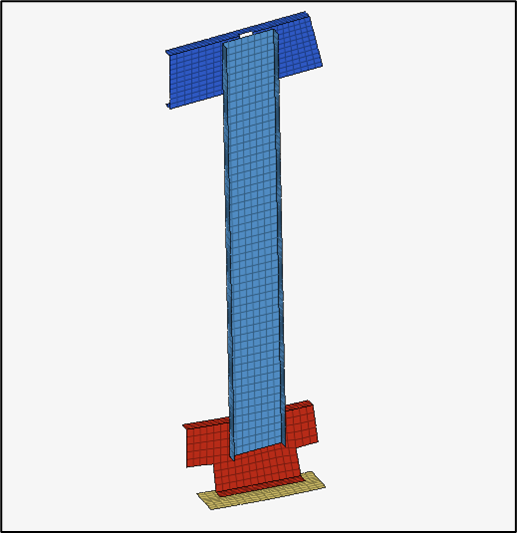
Create the DMIG Output Request
All the matrices in the .h3d file are used in the analysis by default.
-
Press Control
+F or use the
 icon.
icon.
- In the search box, enter ASSIGN.
-
Under Keywords in the search results, select ASSIGN and
press Enter.
An ASSIGN control card is created.
- For Type, select H3DDMIG.
- For matrixname(1), enter DMIG.
-
Point to airframe_section_SUPERELEMENT_CMS.h3d.
Matrices stored in .h3d file are named on retrieval.
Submit the Residual Job
The superelement created by the generation run is utilized in the residual run. The reduced mass, stiffness, and damping matrices, depending on the type of run, are included with the residual structure. The results are obtained at the requested residual structure grids, elements, other attributes, and at the interface points.
- From the menu bar, select Analyze.
-
On the Analyze ribbon, under the Analyze tool group, select Run
OptiStruct Solver
 .
The panel area opens.
.
The panel area opens. - Click Save as.
-
For File name, enter
airframe_section_RESIDUAL.CMS.fem.
The .fem extension is necessary to recognize this as an input file.
- Click Save.
- Set export options: to all.
- Set run options: to analysis.
-
Click Run.
If the job is successful, new results files appear in the directory where Altair HyperWorks was invoked. The airframe_section_RESIDUAL_CMS.out file is a good place to look for error messages to help debug the input deck if any errors are present.The default files written to the directory are:
- airframe_section_RESIDUAL_CMS.html
- HTML report of the analysis giving a summary of the problem formulation and the results.
- airframe_section_RESIDUAL_CMS.out
- ASCII based output file of the model check run before the simulation begins and gives nonlinear iteration history as well as basic information on the results of the run.
- airframe_section_RESIDUAL_CMS.h3d
- HyperView binary results file.
- airframe_section_RESIDUAL_CMS.stat
- Summary of the analysis process, providing CPU information for each step during the analysis process.
View Results
After the analysis:
- Compare the Frequency and Eigenvalue of the residual and baseline models
- Plot the Eigen mode (mag) contours in HyperMesh.
- Open the .out files for both the residual and baseline models (airframe_section_RESIDUAL_CMS.out and airframe_section_BASELINE_CMS.out).
-
Observe the match between Frequency and Eigenvalue of both models.
Figure 2. Comparison of Frequency and Corresponding Eigenvalue Results of Both Models 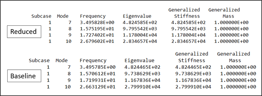
-
In HyperMesh, split the results window.
Figure 3. 
-
Load results in the right section of the window.
-
On the Post ribbon, select Results.
Figure 4. 
-
On the Post ribbon, select Contour.
Figure 5. 
-
Click the
 .
.
-
On the Post ribbon, select Results.
-
Load results in the left section of the window.
By default, this section is for HyperView.
-
Click Apply.
The result shows good match between the full model run and the reduced run.
Figure 6. Eigen Mode (mag) Plots for Baseline and Reduced CMS Models 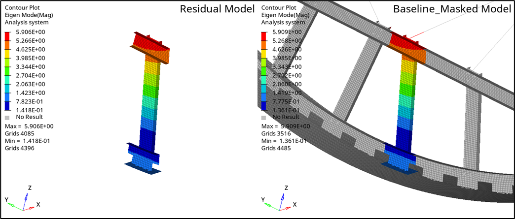
-
Click Apply.