OS-HM-T: 6020 Fatigue Process Manager (FPM) using E-N (Strain - Life) Method
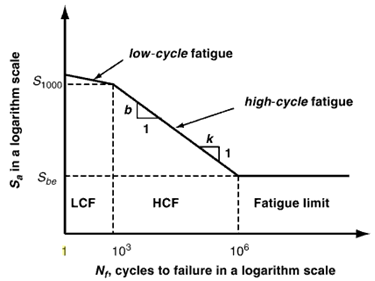
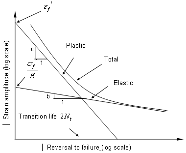
Tutorial Level: Intermediate The E-N (Strain - Life) method should be chosen to predict the fatigue life when plastic strain occurs under the given cyclic loading. S-N (Stress - Life) method is not suitable for low-cycle fatigue where plastic strain plays a central role for fatigue behavior.
In OptiStruct, various strain combination types are available with the default being "Absolute maximum principle strain". In general "Absolute maximum principle stain" is recommended for brittle materials, while "Signed von Mises strain" is recommended for ductile material. The sign on the signed parameters is taken from the sign of the Maximum Absolute Principal value.
In this tutorial, you will be able to evaluate fatigue life with the E-N method.
Launch Altair HyperWorks/HyperMesh and Process Manager
-
Launch Altair HyperWorks from the launch menu.
A New Session dialog is displayed.
- Select the HyperMesh radio button and set Profile to OptiStruct and click the Create Session button.
- From the Templates ribbon, select the Analyze menu and select Fatigue PM.
- For New Session Name, enter <my_session_name>.
- For Working Folder, select your working folder.
-
Click Create.
This creates a new file to save the instance of the currently loaded fatigue process template.
Import the Model
- Make sure the task Import File is selected in the Fatigue Analysis tree.
- For the Model file type, select OptiStruct.
-
Click the Open model file icon
 .
A Select File browser window opens.
.
A Select File browser window opens. - Select the ctrlarm.fem file you saved to your working directory and click Open.
-
Click Import.
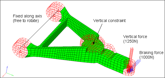
This loads the control arm model. It includes a whole definition of two static subcases, elements sets, and material static properties, etc.
-
Click Apply.
This guides you to the next task Fatigue Subcase of the Fatigue Analysis tree.
Figure 7. Import a Finite Element Model file 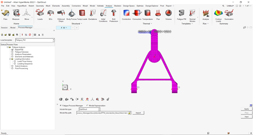
Set Up the Model
Create a Fatigue Subcase
- Make sure the task Fatigue Subcase is selected in the Fatigue Analysis tree.
- In the Create new fatigue subcase field, enter fatsub_fpmtut.
- Click Create.
-
For the Select existing fatigue subcase field, select the newly created fatigue
subcase fatsub_fpmtut.
fatsub_fpmtut is selected as the active fatigue subcase. Definitions in the following processes (analysis parameters, fatigue elements and properties, loading sequences, etc.) will be for this subcase.
- Optionally, you can choose to create all fatigue solver cards (such as FATPARM, FATDEF, FATEVNT, PFAT etc. that are created in subsequent steps) in a separate include file. For this, you should select the check box Create include file for fatigue solver cards (optional).
-
Click Apply.
This saves the current definitions and guides you to the next task Analysis Parameters of the Fatigue Analysis tree.
Figure 8. Create and Select Active Fatigue Subcase to Process 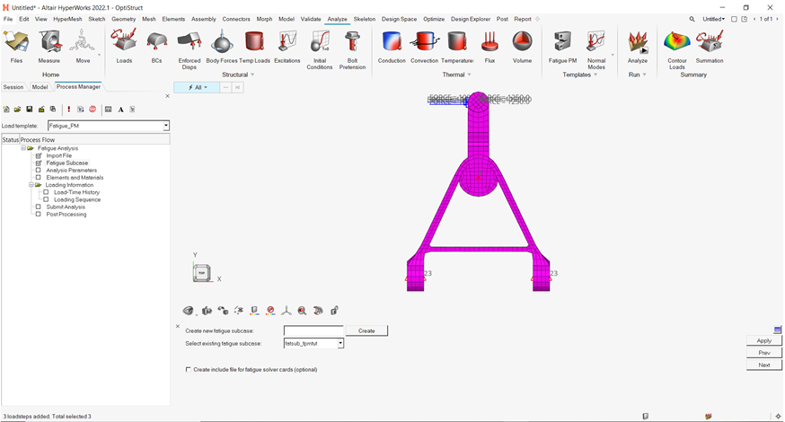
Apply Fatigue Analysis Parameters
- Make sure the task Analysis Parameters is selected in the Fatigue Analysis tree.
- Select the following options:
- Analysis type
- E-N
- Stress combination method
- Signed von Mises
- FEA model unit
- MPA
- Mean stress correction
- SWT
- Rainflow type
- STRESS
- Plasticity correction
- NEUBER
- Enter the following values:
- Certainty of survival
- 0.5
- Gate
- 0.0
-
Click Apply.
This saves the current definitions and guides you to the next task Elements and Materials of the Fatigue Analysis tree. For details, consult the Altair HyperWorks 2025.1 help.
Figure 9. Fatigue Analysis Parameters Definition 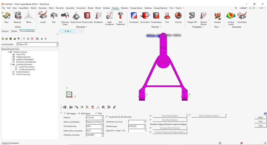
Add Fatigue Elements and Materials
- Make sure the task Elements and Materials is selected in the Fatigue Analysis tree.
-
Click Add Material.
A Material Data window opens.
- For Material name, select Aluminum.
- Make sure Stress unit is set to MPA.
- For Ultimate tensile strength (UTS), enter 600.
-
For Input method of Define EN Curve, select Estimate From
UTS.
Figure 10. Material Data Definition 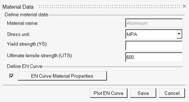
-
Click the Show EN curve definition icon
 .
An EN method description window introducing how to generate the EN material parameter opens.
.
An EN method description window introducing how to generate the EN material parameter opens.Figure 11. EN Curve Material Definition 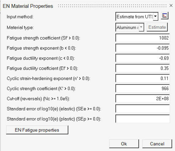
- Click Close.
-
For Material type, select Aluminum and Titanium Alloys
and click Estimate.
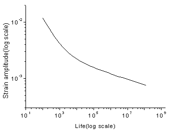
All the data for EN curve definition are automatically estimated.
- Click Plot EN Curve at the bottom of the window to show the EN curve.
- Close the EN Curve plot window.
-
Click Save to save the definition of the EN data for the
selected entities.
Figure 12. 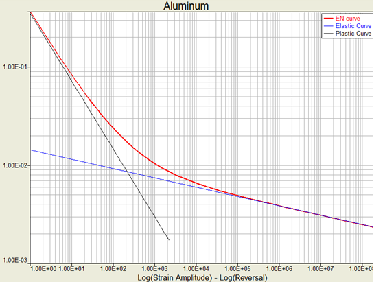
-
Click Add Property.
A Property Data window opens.
- For Property Type, select Property - PSHELL.
-
For Property name, select shell.
This is the skin coating the solid control arm.
- Click Create to create PFAT property.
- For LAYER, select TOP.
- For FINISH, select NONE.
- For TREATMENT, select NONE.
- Leave the field after KF (Fatigue strength reduction factor) set to 1.0.
- Click Close to save the definition of the EN data for the selected elements.
-
Click Apply.
This saves the current definitions and guides you to the next task Load-Time History of the Fatigue Analysis tree.
Figure 13. Property Data Definition 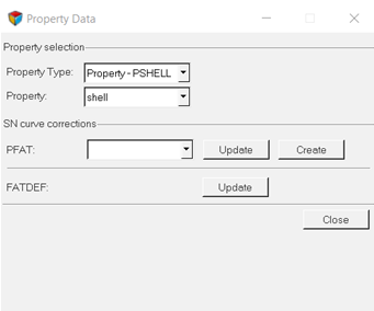
Figure 14. Elements and Material Definition 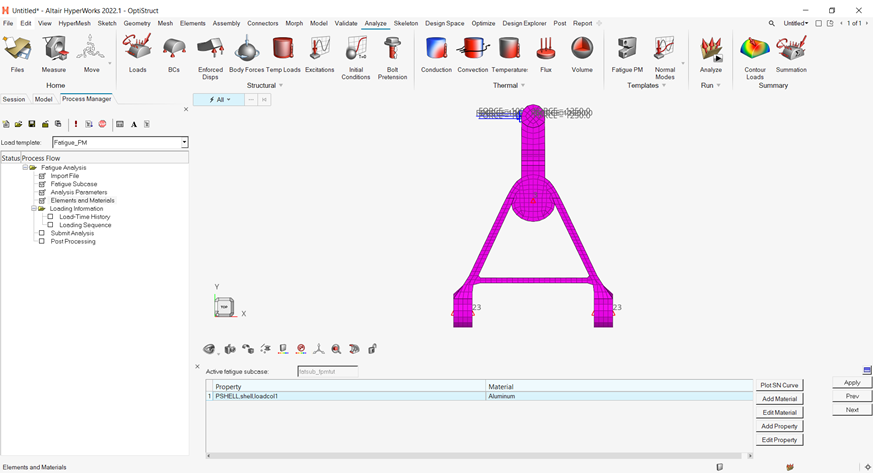
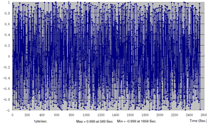
Apply Load-Time History
- Make sure the task Load-Time History is selected in the Fatigue Analysis tree.
-
Click Add by File.
A Load Time History window opens.
- For Load-time history name, enter LTH1.
- For Load-time history type, select CSV.
-
Click the Open load-time file icon .
An Open file browser window opens.
- Browse for load1.csv.
- Click .
-
Click Save to write the new load-time history into
HyperMesh database.
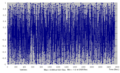
-
Create another load-time history LTH2 by importing the
file load2.csv.
Figure 15. Import Load-Time History 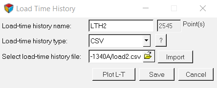
- Click Plot L-T to show the load-time history.
- Close the Load Time History window.
-
Click Apply.
This saves the current definitions and guides you to the next task Loading Sequences of the Fatigue Analysis tree.
Figure 16. Load-Time History Definition 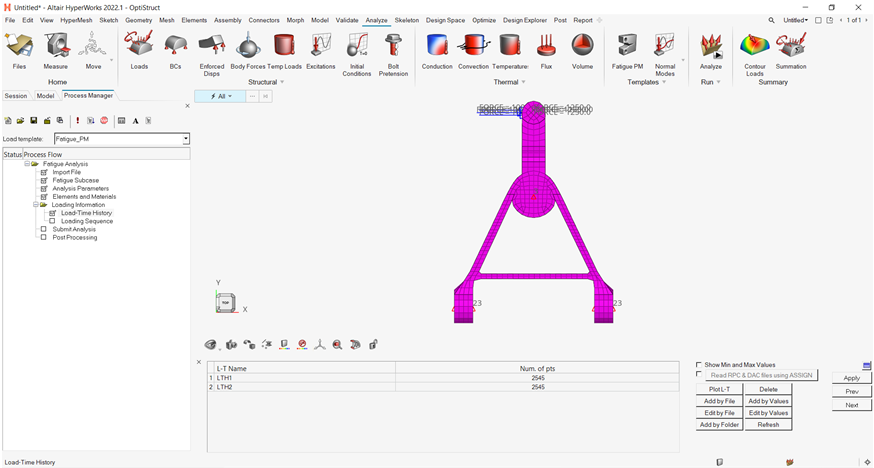
Load Sequences
- Make sure the task Loading Sequences is selected in the Fatigue Analysis tree.
-
Click Add.
A Load Mapping window opens.
- For Channels, select LTH1 and LTH2.
- For Subcase, select SUBCASE1 and SUBCASE2.
- Activate the radio button Auto and leave the event creation method set to default Single Event.
- Click + to create a single event with two subcases and two channels.
-
Set Scale to 5.0, as shown below.
Figure 17. Load Mapping to associate load-time history with static subcase 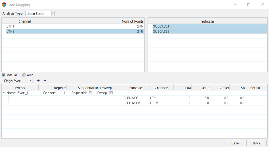
-
Click Save to close the window and create the fatique
event using selected subcases and channels.
Figure 18. Loading Sequences Definition 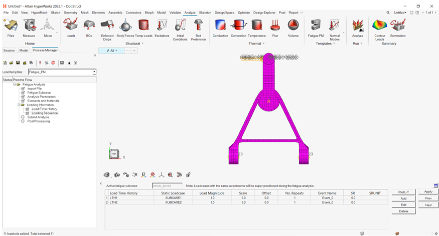
Submit the Job
- Make sure the task Submit Analysis is selected in the Fatigue Analysis tree.
-
Click the Save .fem file icon .
A Save As browser window opens.
- Set the directory in which to save the file, and for File name, enter ctrlarm_fpmtut.fem.
- Click Save to close the window.
- Click Save to save the OptiStruct model file.
- For Run Option, select analysis.
-
Click Submit.
This launches OptiStruct 2025.1 to run the fatigue analysis. If the job is successful, the new results files should be in the directory from which ctrlarm_fpmtut.fem was selected.The default files written to the directory are:
- ctrlarm_fpmtut.0.3.fat
- An ASCII format file which contains fatigue results of each fatigue subcase in iteration step.
- ctrlarm_fpmtut.h3d
- Hyper 3D binary results file, with both static analysis results and fatigue analysis results.
- ctrlarm_fpmtut.out
- OptiStruct output file containing specific information on the file set up, the set up of your fatigue problem, compute time information, etc. Review this file for warnings and errors.
- ctrlarm_fpmtut.stat
- Summary of analysis process, providing CPU information for each step during analysis process.
Note: The filename.#.fat is created for each fatigue subcase at the first and last iterations only if a fatigue optimization is performed.Figure 19. Submit Fatigue Analysis 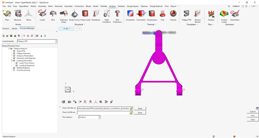
Post-process the Analysis
-
Make sure the task Post-processing is selected in the Fatigue Analysis
tree.
When fatigue analysis has completed successfully after the previous submit, it will automatically go into this task.
- For Fatigue subcase, make sure Select Subcase is selected.
- For Result Type and Data Component, select the required data you want to contour from the drop-down menu.
-
Click Load H3D Results (HV).
This launches HyperView and loads the ctrlarm_fpmtut.h3d results file. It applies the result contour for selected result type and component. You can use HyperView for more detailed results.
-
Click Exit to unload Fatigue Process Manager.
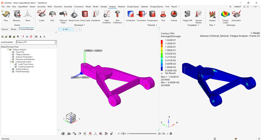
Figure 20. Post-Processing 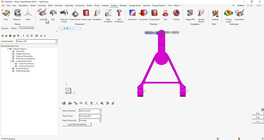
Figure 21. Damage Contour in HyperView