OS-V: 1210 Contact with Friction

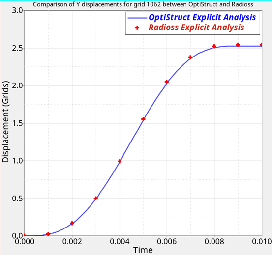
A deformable block is slid over a fixed rigid plate using enforced velocities and the problem is solved using an explicit dynamic analysis in OptiStruct. The results from OptiStruct are compared with an equivalent model in Radioss.

Model Files

Before you begin, copy the file(s) used in this problem to your working directory.

contact_with_friction.fem

Benchmark Model

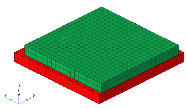
The finite element model consists of a deformable block on which enforced velocities are applied causing it to slide over a rigid fixed block.

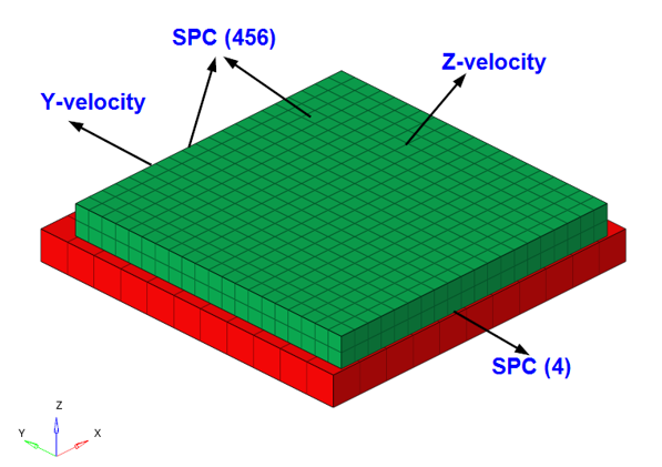
Both blocks are meshed with first-order CHEXA elements and frictional contact is defined between the blocks with a friction coefficient of 0.05. The bottom block is constrained in all directions. One side of the top block is constrained along the Y direction, while the opposite side is subjected to an enforced velocity and constrained along the X, Y, and Z rotational degrees of freedom. The upper side of the top block is subjected to an enforced velocity and is constrained along the X, Y, and Z rotational degrees of freedom.

The Y and Z directional velocities are applied in the form of a sinusoidal variation as a function of time (

t

) given by:(1)

V = \frac{V_{m}}{2} [1 + \sin (\frac{2 π}{T} t + \frac{3 π}{2})] m m / s

Where,

V_{m}

and

T

for Y and Z velocities are:

Direction	$V_{m}$	$T$
Y	565 mm/s	0.009 s
Z	-102 mm/s	0.001 s

The material properties are

Property: Value
Elastic modulus: 193000 N/mm²
Poisson’s ratio: 0.3
Density: 7.75 E-09 tonn/mm³

Results

The Y displacement results are compared between OptiStruct and Radioss at a node on the side where Y-velocity is applied. They seem to be in good agreement (Figure 3).