MV-2110: Use an NLFE Helical Spring in a Cam-Follower Mechanism
Tutorial Level: Advanced In this tutorial, you will learn how to use a pre-defined NLFE Helical Spring sub-system
component in a model.
Before you begin, copy the
CamFollower_stg1.mdl and CamProfile.h3d
files, located in the
mbd_modeling\nlfe\helicalspring folder, to your
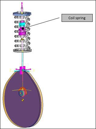
<working directory>.You will learn this process by replacing the traditional coil spring in a Cam
follower mechanism. Figure 1.
What Are NLFE Components in MotionView?
You can add NLFE bodies in MotionView version
14.0 (onwards) using the traditional Body icon in toolbars or through the
browser. In addition to this, ready-to-use subsystems or Components have
been provided. These are components (MotionView
system definition) that can be added to the model using very few user inputs
such as, for example for a Helical Spring: wire diameter, coil diameter,
material properties, number of coils, etc. MotionView will automatically create the building
block entities (such as points, bodies, and joints) and standard outputs
needed to represent such a subsystem.
The following components are made
available:
Helical Spring
Stabilizer Bar
Belt-Pulley
Why Use an NLFE Spring?
An NLFE sub-system offers the following advantages:
The spring component is added as a body, which means the mass and
inertia of the spring is included in the model.
The dynamics induced by the mass of the spring can be modeled and
simulated (for example, surge in springs).
If the deformations in the model are likely to go beyond the linear
assumptions, NLFE will account for it.
Stress strain and deformation contours can be visualized.
Coil-to-coil clash is modeled automatically.
Review the Model
In this step, you will review the provided cam follower model.
Start a new MotionView session.
Load the CamFollower_stg1.mdl file from your
<working directory>.
Review the model.
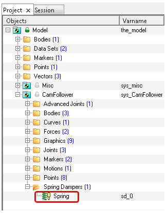
In the Project Browser, the Model is organized using a
CamFollower system, which contains the following:
A Cam, Follower, Joints, Graphics, and a Spring which make the complete
topology.
The spring with a pre-load is acting between the Follower and Ground
Body.
Figure 2. Browser showing the model topology
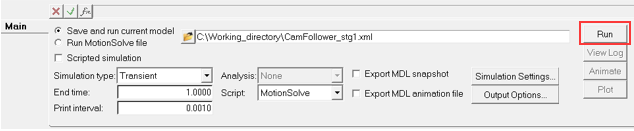
Click the (Run) icon. In the panel, specify the settings shown in
Figure 3. Then click
Run.
Figure 3.
You will use the results from this initial run to compare with the NLFE spring
model results.
When the solver is finished, click Animate to visualize
the animation.
Add an NLFE Helical Spring
In this step, you will replace the coil spring with an NLFE Helical spring
component.
In the Project Browser, right-click on the
Spring and select Deactivate > Selected and dependents from the context menu.
Figure 4.
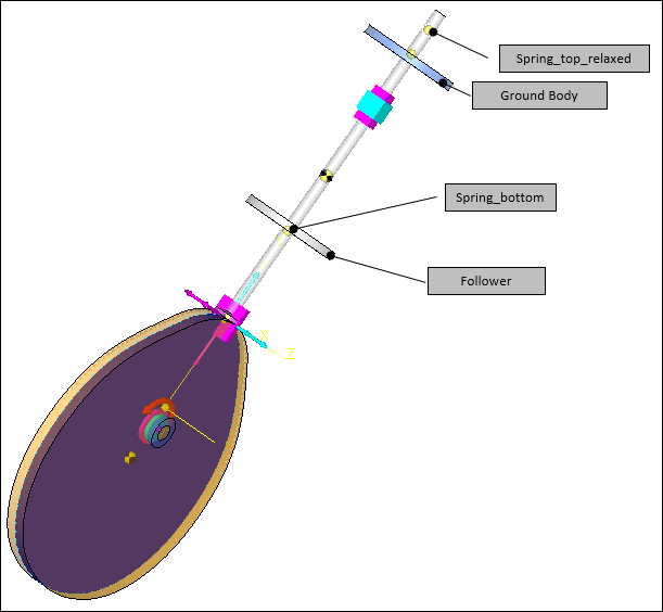
You will add the NLFE spring between the Ground Body (on top) and the Follower
(at the bottom). The corresponding points you will use are Spring_top_relaxed
and Spring_bottom. Figure 5.
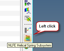
In the Subsystems toolbar, click (NLFE Helical Spring Subsystem).
Figure 6.
Tip: This toolbar may not be turned on by default. From the menu bar, click View > Toolbars > MotionView and then click on the toolbar name to turn the display
on/off.
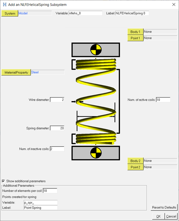
In the Add an NLFEHelicalSpring Subsystem dialog, assign
an appropriate Label and Variable.
Figure 7.
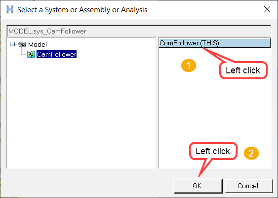
Double-click on the parent System collector to bring up
the Model Tree. Select
CamFollower as the parent system.
Figure 8.
Resolve the other collectors.
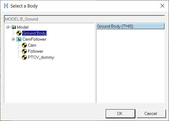
For , select Ground
Body.
Figure 9.
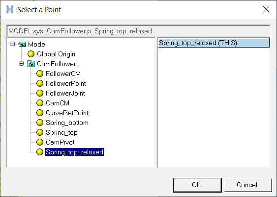
For , select
Spring_top_relaxed.
Figure 10.
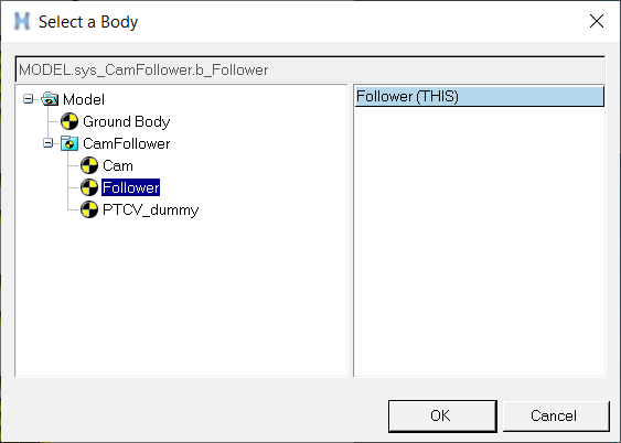
For , select
Follower.
Figure 11.
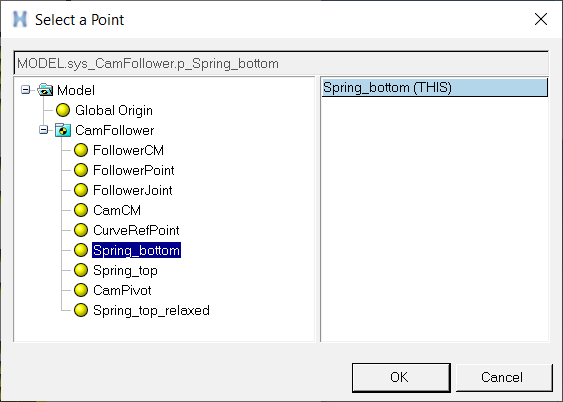
For , select
Spring_bottom.
Figure 12.
For , select Steel.
Figure 13.
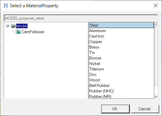
Fill in the spring parameters and details for label and varnames as shown in
Table 1. Then click
OK.
Table 1.
Spring Parameters
Wire diameter
Specify the coil spring wire diameter.
3
Spring diameter
Specify the coil mean diameter: center-tocenter.
20
Num. of inactive coils
Specify the inactive/dead coils at each end.
1
Num. of active coils
Specify the active coils which contribute to spring
stiffness.
7
Additional Parameters
Number of elements per coils
Specify the element density per coil.
10
Variable
Specify varname prefix for the spring profile points
created.
p_spr_
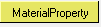
Label
Specify label prefix for the spring profile points
created.
Point Spring
Note: These parameters have been chosen for the following reasons:
The stiffness of the coil spring being replaced is: 14.6 N/mm.
The equation for the coil spring stiffness:
G.d4/[8.n.D3] (Where: G = Modulus of
rigidity; d = Wire dia.; n = No. of active coils; D = Spring mean
diameter).
Substituting the values from the table above in the equation and
using Steel with 80769 N/mm2 for material: Spring
stiffness k = 80769x34/[8x7x203] = 14.6
N/mm.
Figure 14.
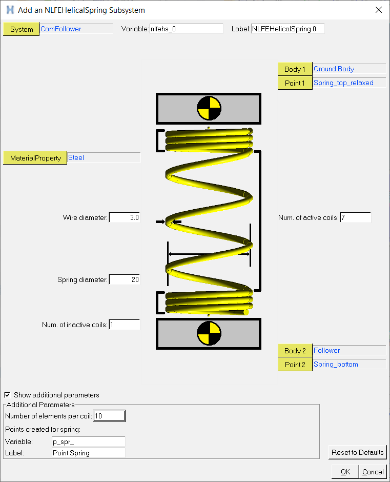
The spring will be added between the Follower and Ground Body. Figure 15. The spring overshoots the upper plate as shown in Figure 15. This is because
the spring has been created with no pre-load on it.
Review the NLFE Spring systems added.
The following entities are available in the system:
An NLFE Spring.
DataSet with spring parameters that were used to create the spring.
Fixed joints connecting the spring to the suspension.
Markers for reference.
Points that define the spring profile.
Template with unsupported elements. These are automatically created and
include elements that define coil-to-coil contacts.
Figure 16. NLFE spring topology in the browser
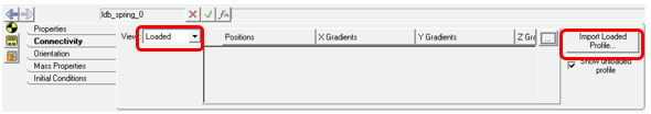
Add the pre-loaded positions for the spring.
Under the subsystem, select the NLFE Spring 0
body to open the body panel.
From the Connectivity tab, in the View drop-down
menu select the Loaded option.
This will show the Import Loaded Profile button, which you can
use to load a .csv file containing the pre-loaded
positions and gradients of the spring.
Click the Import Loaded Profile button.
Figure 17. NLFE Connectivity tab - Loaded View
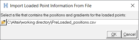
In the Import Loaded Points Information From File
dialog, browse to your <working directory> and
select PreLoaded_positions.csv.
Figure 18.
Click OK to import
the loaded positions.
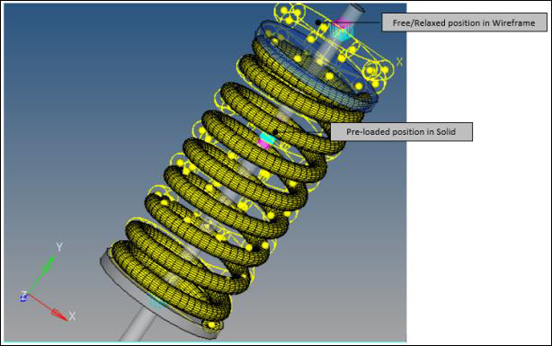
The spring will be displayed in wireframe and solid. The one in
wireframe is the No Load position (free/relaxed configuration) and the
solid representation is that of pre-loaded spring.
Note: Refer to the
Appendix in the NLFE Body Panel – Connectivity Tab
topic to learn how you can generate a preloaded position CSV
file.
Figure 19. Free/Relaxed and Pre-loaded position of the spring
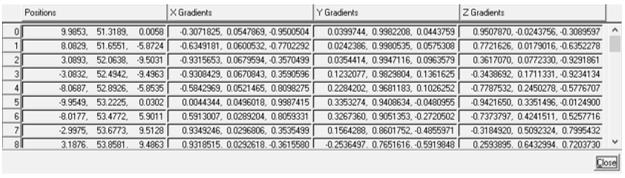
Click the (Expansion) button to view the pre-loaded
positions.
Figure 20. Pre-loaded positions and gradients imported from the .csv
file The fixed joints created by the NLFEHelicalSpring Component utility will
be at the free positions. You need to move one of these to the pre-loaded
positions. Inspecting the spring positions reveals that the spring is compressed
at the top while the bottom position is the same in both the
configurations.
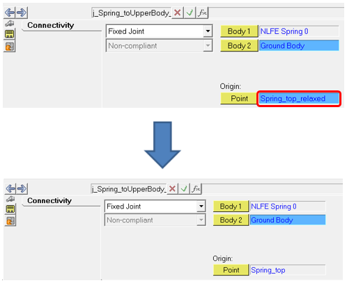
Change the origin point of the joint Spring_toUpperBody_att in the NLFE Helical
Spring 0 system from Spring_top_relaxed to Spring_top (in
the parent CamFollower system).
Under Origin, double-click the Point collector
to display the model tree.
Clear the Only show entities within valid scope
check box.
Select Spring_top using the model tree or in the
graphics area (after closing the model tree).
Figure 21. Changing the connection to pre-loaded position
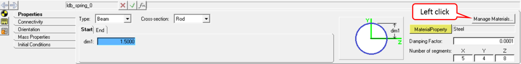
From the Properties tab, click Manage Materials.
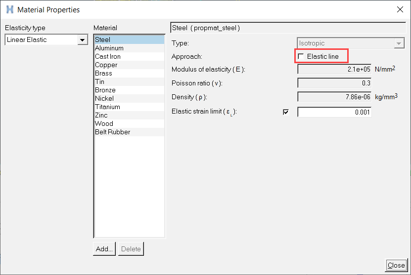
The Material Properties dialog opens.Figure 22.
Deselect the Elastic Line check box to capture
non-linear effects due to deformation of the spring.
The Elastic Line check box is selected by default for the Steel material.Figure 23.
Click Close to exit the Material
Properties dialog.
Click and save the model as
CamFollower_nlfe.mdl.
Solve and Post-Process the Model
In this step, you will solve the model and plot the results.
Click the (Run) panel icon.
Specify a name for the .xml file and click on the
Run button.
After the simulation is completed, click on the Animate
button to view the animation in HyperView.
Use the (Start/Pause Animation) button
to play the animation.
You can see coil-to-coil clash at the bottom/top set of coils: Figure 24. Coil-to-coil contact visualization in HyperView
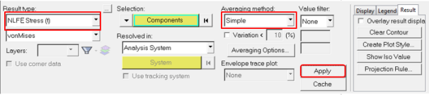
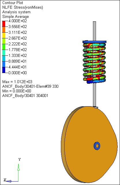
Click the (Contour panel) icon to activate
the Contour panel.
In the panel, for Result type select NLFE Stress (t) and
for Averaging method select Simple. Then click
Apply.
Figure 25. Viewing results in HyperViewThis will allow you to view the stress contours.
Figure 26. Contours in HyperView
Note: You can also view Displacement, Strain, etc. for an NLFE body in HyperView. All FE contours and types are available
for an NLFE body.
Compare Results
Now you will compare the results from the NLFE spring and the regular
spring.
Click to add a new page.
Change the client to HyperGraph 2D.
On the Page Window Layout toolbar, click > to split the window.
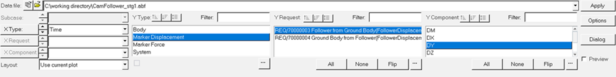
In the left window, click and load the .abf file
corresponding to the solver run with the original spring (created in the step
Review the Model). Make the selections for the
plot shown in Table 2
then click Apply.
Table 2.
X Type
Time
Layout
Use current plot
Y Type
Marker Displacement
Y Request
REQ/70000003 Follower from Ground
Body(FollowerDisplacement)
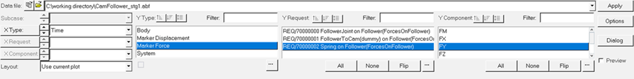
In the right window, make the selections in Table 3 and click
Apply.
Table 3.
X Type
Time
Layout
Use current plot
Y Type
Marker Force
Y Request
REQ/70000002 Spring on
Follower(ForcesOnFollower)
Y Component
FY
Figure 28. Plot selections – Spring force on follower: regular spring
In the left window, browse to the .abf file (created in
step 4) to plot
the corresponding displacement for the NLFE results.
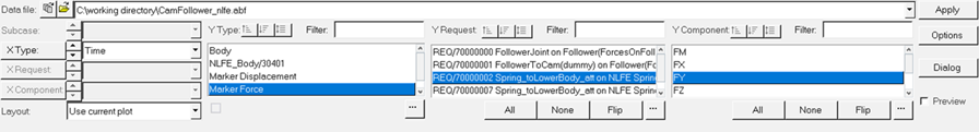
In the right window, make the selections shown in Table 4 and click
Apply.
Table 4.
X Type
Time
Layout
Use current plot
Y Type
Marker Force
Y Request
REQ/70000002 Spring_toLowerBody_att on NLFE
Spring0(ForcesOnFollower)
Y Component
FY
Figure 29. Plot selections – Spring force on follower: NLFE spring
Apply axis labels and formatting as appropriate.
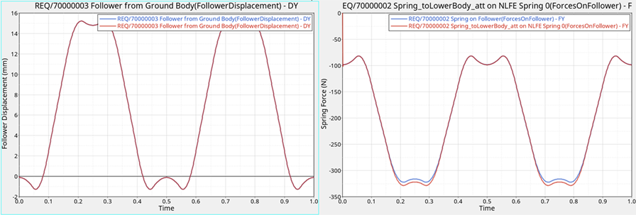
The comparison is shown in Figure 30:Figure 30. Result comparison: Regular spring versus NLFE spring
Upon closer inspection there are some differences in the results, especially
in the Spring Forces. These could be attributed to the following reasons:
NLFE spring has mass and inertias associated with it as it is
represented as a body. A regular spring is a force entity without any
mass/inertias.
The difference in force outputs is particularly seen when the spring
displacement is high. This is the point where the coil-to-coil contact
happens. During this event, the effective number of coils reduces, thus
increasing the spring stiffness marginally and hence the force
outputs.
Click and save your work in a session
file named camfollower_nlfe.mvw.

 (Run) icon. In the panel, specify the settings shown in
Figure 3. Then click
Run.
(Run) icon. In the panel, specify the settings shown in
Figure 3. Then click
Run.
 You will use the results from this initial run to compare with the NLFE spring model results.
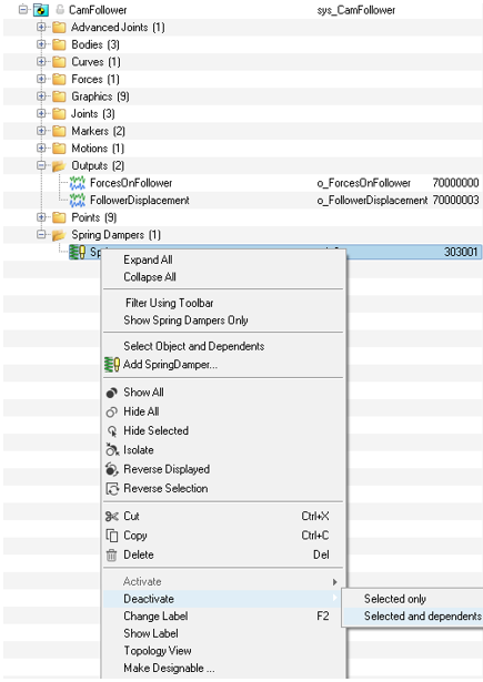
 (NLFE Helical Spring Subsystem).
 , select Ground
Body.
, select Ground
Body.
 , select
Spring_top_relaxed.
, select
Spring_top_relaxed.
 , select
Follower.
, select
Follower.
 , select
Spring_bottom.
, select
Spring_bottom.
 , select Steel.

 (Expansion) button to view the pre-loaded
positions.
(Expansion) button to view the pre-loaded
positions.
 and save the model as
CamFollower_nlfe.mdl.
and save the model as
CamFollower_nlfe.mdl.
 (Start/Pause Animation) button
to play the animation.
You can see coil-to-coil clash at the bottom/top set of coils:
(Start/Pause Animation) button
to play the animation.
You can see coil-to-coil clash at the bottom/top set of coils: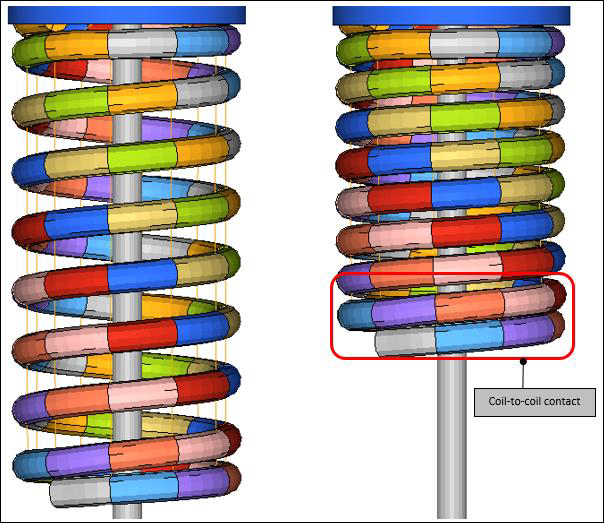
 (Contour panel) icon to activate
the Contour panel.
(Contour panel) icon to activate
the Contour panel.
 to add a new page.
 .
.
 >
>  to split the window.
 and load the .abf file
corresponding to the solver run with the original spring (created in the step
Review the Model). Make the selections for the
plot shown in Table 2
then click Apply.
and load the .abf file
corresponding to the solver run with the original spring (created in the step
Review the Model). Make the selections for the
plot shown in Table 2
then click Apply.
 and save your work in a session
file named camfollower_nlfe.mvw.
and save your work in a session
file named camfollower_nlfe.mvw.