The S-N curve, first developed by Wöhler, defines a relationship between stress and
number of cycles to failure.
Typically, the S-N curve (and other fatigue properties) of a material is obtained
from experiment; through fully reversed rotating bending tests. Due to the large
amount of scatter that usually accompanies test results, statistical
characterization of the data should also be provided (certainty of survival is used
to modify the S-N curve according to the standard error of the curve and a higher
reliability level requires a larger certainty of survival).Figure 1. S-N Data from Testing
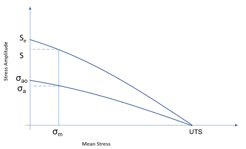
When S-N testing data is presented in a log-log plot of alternating nominal stress
amplitude or range versus cycles to failure , the relationship between and can be described by straight line segments.
Normally, a one or two segment idealization is used.Figure 2. One Segment S-N Curves in Log-Log Scale
for segment 1
Where, is the nominal stress range, are the fatigue cycles to failure, is the first fatigue strength exponent, and is the fatigue strength coefficient.
The S-N approach is based on elastic cyclic loading, inferring that the S-N curve
should be confined, on the life axis, to numbers greater than 1000 cycles. This
ensures that no significant plasticity is occurring. This is commonly referred to as
high-cycle fatigue.
S-N curve data is provided for a given material using the Materials module.
Multiple SN Curves
HyperLife supports the following Multiple SN curve types:
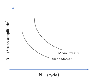
Multi-mean S-N curves: group of S-N curves defined at different mean
stress.
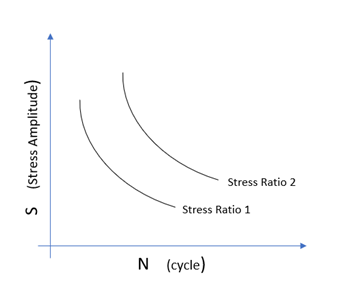
Multi-ratio S-N curves: group of S-N curves defined at different stress
ratio R.
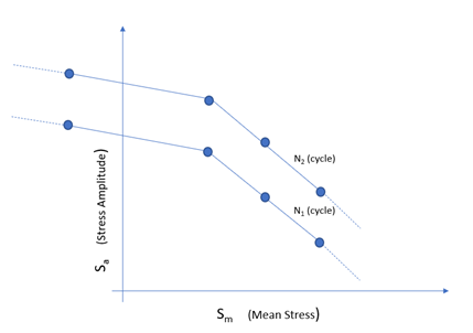
Multi-Haigh Diagram: group of Haigh curves defined at different Number of
Cycles.
Note: Refer Mean Stress = Interpolate, to understand how life is determined
when Multiple SN curves are assigned.
Rainflow Cycle Counting
Cycle counting is used to extract discrete simple "equivalent" constant amplitude
cycles from a random loading sequence.
One way to understand "cycle counting" is as a changing stress-strain versus time
signal. Cycle counting will count the number of stress-strain hysteresis loops and
keep track of their range/mean or maximum/minimum values.
Rainflow cycle counting is the most widely used cycle counting method. It requires
that the stress time history be rearranged so that it contains only the peaks and
valleys and it starts either with the highest peak or the lowest valley (whichever
is greater in absolute magnitude). Then, three consecutive stress points (1, 2, and
3) will define two consecutive ranges as and . A cycle from 1 to 2 is only extracted if . Once a cycle is extracted, the two points forming
the cycle are discarded and the remaining points are connected to each other. This
procedure is repeated until the remaining data points are exhausted.
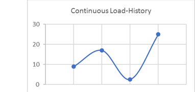
Simple Load History
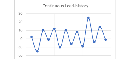
Figure 6. Continuous Load History
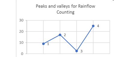
Since this load history is continuous, it is converted into a load history consisting
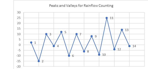
of peaks and valleys only.Figure 7. Peaks and Valleys for Rainflow Counting. 1, 2, 3, and 4 are the four peaks and valleys
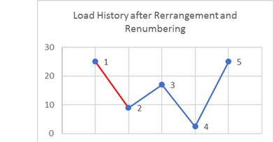
It is clear that point 4 is the peak stress in the load history, and it will be moved
to the front during rearrangement (Figure 8). After rearrangement, the peaks and
valleys are renumbered for convenience.Figure 8. Load History after Rearrangement and Renumbering
Next, pick the first three stress values (1, 2, and 3) and
determine if a cycle is present.
If represents the stress value, point then:
As you can see from Figure 8, ; therefore, no cycle is extracted from point 1 to 2.
Now consider the next three points (2, 3, and 4).
, hence a cycle is extracted from point 2 to 3. Now
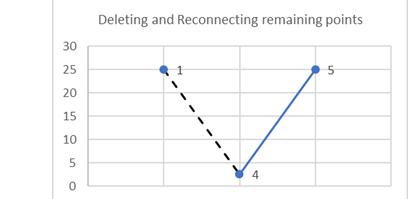
that a cycle has been extracted, the two points are deleted from the graph.Figure 9. Delete and Reconnect Remaining Points
The same process is applied to the remaining points:
In this case, , so another cycle is extracted from point 1 to 4.
After these two points are also discarded, only point 5 remains; therefore, the
rainflow counting process is completed.
Two cycles (2→3 and 1→4) have been extracted from this load history. One of the main
reasons for choosing the highest peak/valley and rearranging the load history is to
guarantee that the largest cycle is always extracted (in this case, it is 1→4). If
you observe the load history prior to rearrangement, and conduct the same rainflow
counting process on it, then clearly, the 1→4 cycle is not extracted.
Complex Load History
The rainflow counting process is the same regardless of the number of load history
points. However, depending on the location of the highest peak/valley used for
rearrangement, it may not be obvious how the rearrangement process is
conducted.Figure 10 shows just the rearrangement
process for a more complex load history. The subsequent rainflow counting is just an
extrapolation of the process mentioned in the simple example above, and is not
repeated here.Figure 10. Continuous Load History
Since this load history is continuous, it is converted into a load history consisting
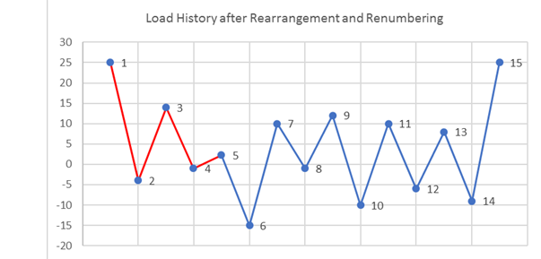
of peaks and valleys only:Figure 11. Peaks and Valleys for Rainflow Counting
Clearly, load point 11 is the highest valued load and therefore, the load history is
now rearranged and renumbered.Figure 12. Load History After Rearrangement and Renumbering
The load history is rearranged such that all points including and after the highest
load are moved to the beginning of the load history and are removed from the end of
the load history.
Complex Load History
Equivalent Nominal Stress
Since S-N theory deals with uniaxial stress, the stress components need to be
resolved into one combined value for each calculation point, at each time step, and
then used as equivalent nominal stress applied on the S-N curve.
Various stress combination types are available with the default being "Absolute
maximum principle stress". "Absolute maximum principle stress" is recommended for
brittle materials, while "Signed von Mises stress" is recommended for ductile
material. The sign on the signed parameters is taken from the sign of the Maximum
Absolute Principal value.
"Critical plane stress" is also available as a stress combination for uniaxial
calculations (stress life and strain life).
Normal Stress resolved at each plane is
calculated by:
HyperLife expects a number of planes (n) as input, which are
converted to equivalent using the following formula.
For example, if number of planes requested is 20, then stress is calculated every 10
degrees.
By default, HyperLife also calculates at = 45 and 135-degree planes in addition to the
requested number of planes. This is to include the worst possible damage if
occurring on these planes.
Mean Stress Correction
Generally, S-N curves are obtained from standard experiments with fully reversed
cyclic loading. However, the real fatigue loading could not be fully-reversed, and
the normal mean stresses have significant effect on fatigue performance of
components. Tensile normal mean stresses are detrimental and compressive normal mean
stresses are beneficial, in terms of fatigue strength. Mean stress correction is
used to take into account the effect of non-zero mean stresses.
The Gerber parabola and the Goodman line in Haigh's coordinates are widely used when
considering mean stress influence, and can be expressed as:
Gerber
When SN curve is of the Stress Ration R = -1
When SN curve is of the Stress Ratio R != -1
Goodman
When SN curve is of the Stress Ratio R = -1
When SN curve is of the Stress Ratio R != -1
Gerber2
Improves the Gerber method by ignoring the effect of negative mean stress.
When SN curve is of the Stress Ratio R != -1
If , same as Gerber
If ,
Soderberg
Is slightly different from GOODMAN; the mean stress is normalized by yield stress
instead of ultimate tensile stress.
When SN curve is of the Stress Ratio R = -1
Where,
Equivalent stress amplitude
Stress amplitude
Mean stress
Yield stress
When SN curve is of the Stress Ratio R != -1
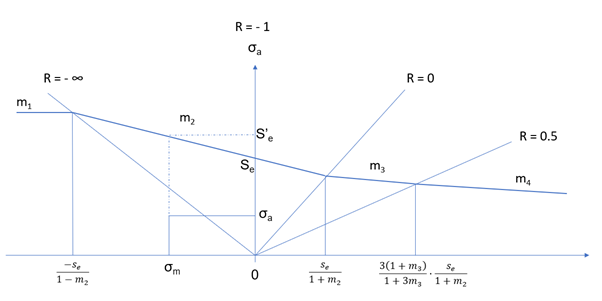
FKM
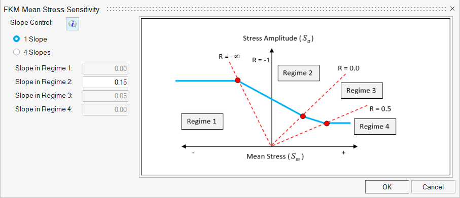
If only one slope field is specified for mean stress correction, the corresponding
Mean Stress Sensitivity value () for Mean Stress Correction is set equal to Slope in
Regime 2 (Figure 14). Based on FKM-Guidelines, the Haigh diagram is divided into
four regimes based on the Stress ratio () values. The Corrected value is then used to choose
the S-N curve for the damage and life calculation stage.Figure 14.
Note: The FKM equations below illustrate the calculation of Corrected Stress
Amplitude (). The actual value of stress used in the Damage
calculations is the Corrected stress range (which is ). These equations apply for SN curves input by
the user (by default, any user-defined SN curve is expected to be input for a
stress ratio of R=1.0).
There are two available options for FKM correction in HyperLife. They are activated by setting FKM MSS to
1 slope/4 slopes in the
Assign Material dialog.
If only one slope is defined and if mean stress correction on an SN module is set to
FKM:
Regime 1 (R > 1.0)
Regime 2 (-∞ ≤ R ≤ 0.0)
Regime 3 (0.0 < R < 0.5)
Regime 4 (R ≥ 0.5)
Where,
Stress amplitude after mean stress correction (Endurance stress)
Mean stress
Stress amplitude
User-inputted mean stress sensitivity M
If all four slopes are specified for mean stress correction, the corresponding Mean
Stress Sensitivity values are slopes for controlling all four regimes. Based on
FKM-Guidelines, the Haigh diagram is divided into four regimes based on the Stress
ratio () values. The corrected value is then used to choose
the S-N curve for the damage and life calculation stage.
If four slopes are defined and mean stress correction is set to
FKM:
User-inputted mean stress sensitivities M1 M2,
M3 and M4
Interpolate
Multi-Mean SN Curves
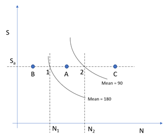
Life is usually determined by interpolation of two SN curves with
respect to mean stress. A log function mentioned below is a 10 base log
function.Figure 15.
Case A
If a cycle has a mean stress of 150MPa at point A, HyperLife locates point 1 and point 2 in Figure 15. Then HyperLife linearly
interpolates logN1 and logN2 with respect to mean stress in order to
determine logN_A at mean stress 150MPa. Once logN_A is determined, life
(N_A) and corresponding damage can be determined.
Case B
If the cycle has a mean stress greater than the maximum mean stress of
the curve set (180MPa in this case), HyperLife offers two options to choose its behavior.
Option 1 , Curve Extrapolation = False
Use an SN curve of the maximum mean stress (the SN curve of
mean stress 180 MPa in this case). In the example in
HyperLife, N1 is the life
HyperLife will report.
Option 2 , Curve Extrapolation = True
Extrapolate log(N) of the two SN curves with the highest
mean stress values. In the example in Figure 15, log(N) will be extrapolated from
log(N1) and log(N2) with respect to mean stress.
Case C
If the cycle has a mean stress less than the minimum mean stress of the
curve set (90MPa in this case), HyperLife
will use the SN curve of the minimum mean stress to determine life. In
the example in Figure 15, life will be N2.
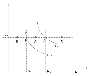
Multi-Stress Ratio SN Curve
Life is usually determined by interpolation of 2 SN curves with respect
to mean stress. When multi-stress ratio SN curves are used, HyperLife assumes that you will not define SN
curves with stress ratio greater than or equal to 1, which are SN curves
with compressive stress or zero stress amplitude. A log function
mentioned below is a 10 base log function. R denotes a stress ratio.Figure 16.
Case A
If a cycle has R = -0.2 at point A, HyperLife locates point 1 and point 2 in Figure 16. Then HyperLife linearly
interpolates logN1 and logN2 with respect to mean stress in order to
determine logN_A at R = -0.2. Once R value and stress amplitude of the
cycle are given, we can always calculate mean stress of the cycle. Once
logN_A is determined, life (N_A) and corresponding damage can be
determined. It is worthwhile to mention that HyperLife does not use stress ratio for
interpolation because R can be an infinite value when maximum stress is
zero.
Case B
If the cycle has R greater than the maximum R of the curve set (R=0 in
this case), HyperLife offers two options to
choose its behavior.
Option 1, Curve Extrapolation = False
Use an SN curve of the maximum R (the SN curve of R= 0 in
this case). In the example in Figure 16, N1 is the life HyperLife will report.
Option 2, Curve Extrapolation = True
Extrapolate log(N) of the two SN curves with the highest R
values. In the example in Figure 16, log(N) will be extrapolated from
log(N1) and log(N2) with respect to mean stress.
Case C
If the cycle has R less than the minimum R of the curve set (R= -1 in
this case), HyperLife will use the SN curve
of the minimum R to determine life. In the example in Figure 16, life will be N2.
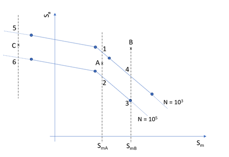
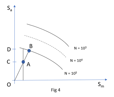
Constant Life Haigh Diagram
Life is usually determined by interpolation of two Haigh diagrams with
respect to stress amplitude. A log function mentioned below is a 10 base
log function.Figure 17.
Interpolation on a Constant Mean Stress Line
If you choose constant mean stress line for linear
interpolation of Haigh diagram, HyperLife interpolates two Haigh
diagrams on a constant mean stress line as described in the following.
Case A
If a cycle has a mean stress and stress
amplitude at point A, HyperLife locates point 1 and
point 2 in Figure 17. Life of point A should be between
1000 and 100000. HyperLife linearly interpolates
log(1000) and log(100000) with respect to stress
amplitude along Sm_A constant mean stress line in
order to determine logN_A at point A. Once logN_A
is determined, life (N_A) and corresponding damage
can be determined.
Case B
If a point (mean stress, stress amplitude) is
located above or below all the Haigh diagrams,
life of the point is calculated by extrapolation
of the two highest or two lowest curves. In the
example in Figure 17, log(1000) and log(100000) will be
extrapolated with respect to stress amplitude
along Sm_B constant mean stress line.
Case C
In this case, stress amplitude at point 5 and
point 6 may be calculated from extrapolation. Once
stress amplitudes become available at the 2
points, a procedure described in case A is
applied.
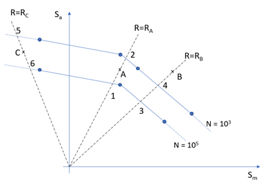
Interpolation on a Constant Stress Ratio Line
Figure 18. If you choose constant stress ration line for linear
interpolation of Haigh diagram, HyperLife interpolates two Haigh
diagrams on a constant stress ratio line as described in the following.
Case A
If a cycle has a mean stress and stress
amplitude at point A, HyperLife locates point 1 and
point 2 in Figure 18. Life of point A should be between
1000 and 100000. HyperLife linearly interpolates
log(1000) and log(100000) with respect to stress
amplitude along RA constant stress ratio line in
order to determine logN_A at point A. Once logN_A
is determined, life (N_A) and corresponding damage
can be determined.
Case B
If a point (mean stress, stress amplitude) is
located above or below all the Haigh diagrams,
life of the point is calculated by extrapolation
of the two highest or two lowest curves. In the
example in Figure 18, log(1000) and log(100000) will be
extrapolated with respect to stress amplitude
along R=RB constant stress ratio line.
Case C
In this case, stress amplitude at point 5 and
point 6 may be calculated from extrapolation. Once
stress amplitudes become available at the 2
points, a procedure described in case A is applied
on constant stress ratio line R=RC.
Damage Accumulation Model
Palmgren-Miner's linear damage summation rule is used. Failure is predicted
when:
Where,
Materials fatigue life (number of cycles to failure) from its S-N curve
at a combination of stress amplitude and means stress level .
Number of stress cycles at load level .
Cumulative damage under load cycle.
The linear damage summation rule does not take into account the effect of the load
sequence on the accumulation of damage, due to cyclic fatigue loading. However, it
has been proved to work well for many applications.
The fatigue life or damage obtained for the event specified can be scaled in HyperLife as shown below. Scaled life or scaled damage will
be available as additional output from the fatigue evaluation.
Life (which is 1/Damage) is scaled in equivalent
units.
Linearly accumulated damage can be modified by applying the
Allowable Miner sum. Scaled life and scaled damage are supported for SN, EN,
Transient Fatigue, Weld Fatigue, and Vibrational Fatigue.
Safety Factor
Safety factor is calculated based on the endurance limit or target stress (at target
life) against the stress amplitude from the working stress history.
HyperLife calculates this ratio via two criteria:
Mean Stress = Constant
Stress Ratio = Constant
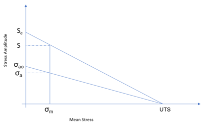
The safety factor (SF) based on the mean stress correction applied is given by the
following equations.
Mean Stress = Constant
Goodman or Soderberg
When SN curve is of the Stress Ratio R =
-1
= Target stress amplitude
against the target life from the modified SN curve
= Stress amplitude after mean
stress correction
Figure 19.
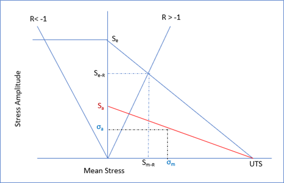
When SN curve is of the Stress Ratio R != -1Figure 20.
= Stress Amplitude
= Mean Stress
= Endurance limit obtained from
SN curve with R ratio
= Mean Stress corresponding to
If ,
If ,
If ,
If ,
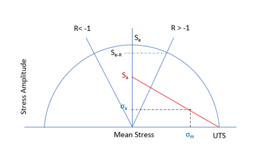
Gerber
Figure 21. When SN curve is of the Stress Ratio R != -1Figure 22.
Gerber2
When SN curve is of the Stress Ratio R != -1
If
If ,
If ,
If ,
FKM
Figure 23.
No Mean Stress Correction
Stress Ratio = Constant
Goodman
When SN curve is of the Stress Ratio R = -1
Figure 24.
When SN curve is of the Stress Ratio R != -1
If ,
If ,
If ,
If ,
Gerber
When SN curve is of the Stress Ratio R = -1
When SN curve is of the Stress Ratio R != -1
If ,
If ,
Gerber2
When SN curve is of the Stress Ratio R != -1
If
If ,
If ,
If ,
FKM
= Corrected Stress Amplitude in
Constant R mean stress correction
No Mean Stress Correction
Interpolate
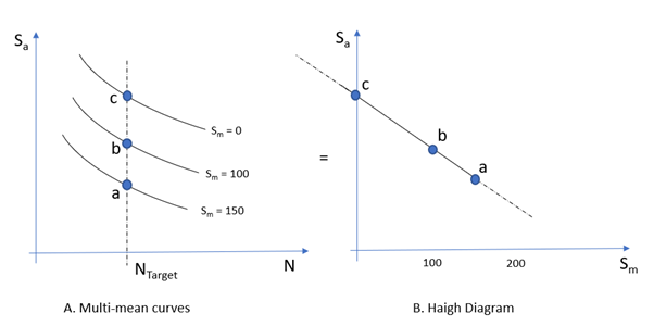
Safety Factor with Multi-Mean
To calculate safety factor, HyperLife creates an internal
Haigh diagram for the target life using multi-mean SN
curve by finding stress amplitude-mean stress pairs at
the target life. Using the internally created Haigh
diagram, HyperLife
calculates safety factor as described in section Safety
Factor in Chapter Haigh diagram. The number of data
points of the Haigh diagram is the number of curves.
Thus the more number of curves, the better result. When
Haigh diagram is not available in mean stress ranges,
HyperLife extrapolates
the Haigh diagram.Figure 25. Conversion of Multi-Mean Curve to Haigh
Diagram
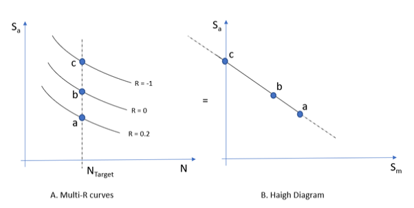
Safety Factor with Multi-Ratio
To calculate safety factor, HyperLife create an internal
Haigh diagram for the target life using multi-mean SN
curve by finding stress amplitude-mean stress pairs at
the target life. The number of data points of the Haigh
diagram is the number of curves. Thus, the more number
of curves, the better result. When Haigh diagram is not
available in mean stress ranges, HyperLife extrapolates the Haigh
diagram.Figure 26. Conversion of Multi-Mean Curve to Haigh
Diagram
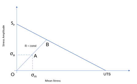
Safety Factor with Haigh
Safety factor (SF) is calculated in the following manner
in Figure 27.Figure 27. When target life is 100000:
Constant R : SF = OB/OA
Constant mean : SF = OD/OC
If Haigh diagram for a target life is not defined,
HyperLife creates Haigh
diagram for the target life. In Figure 27, if target life is 10000, and Haigh
diagram for N=10000 is not defined, HyperLife will created dashed
curve to calculate Safety factor.
Safety Factor with Multi-Mean
To calculate safety factor, HyperLife creates an internal
Haigh diagram for the target life using multi-mean SN curve by finding stress
amplitude-mean stress pairs at the target life. Using the internally created Haigh
diagram, HyperLife calculates safety factor as described
in section Safety Factor in Chapter Haigh diagram. The number of data points of the
Haigh diagram is the number of curves. Thus the more number of curves, the better
result. When Haigh diagram is not available in mean stress ranges, HyperLife extrapolates the Haigh diagram.Figure 28. Conversion of Multi-Mean Curve to Haigh Diagram
Safety Factor with Multi-Ratio
To calculate safety factor, HyperLife create an internal
Haigh diagram for the target life using multi-mean SN curve by finding stress
amplitude-mean stress pairs at the target life. The number of data points of the
Haigh diagram is the number of curves. Thus, the more number of curves, the better
result. When Haigh diagram is not available in mean stress ranges, HyperLife extrapolates the Haigh diagram.Figure 29. Conversion of Multi-Mean Curve to Haigh Diagram
Safety Factor with Haigh
Safety factor (SF) is calculated in the following manner in Figure 30.Figure 30.
When target life is 100000:
Constant R : SF = OB/OA
Constant mean : SF = OD/OC
If Haigh diagram for a target life is not defined by user, HyperLife creates Haigh diagram for the target life. In Figure 30, if target life is 10000, and Haigh diagram for N=10000 is not
defined, HyperLife will created dashed curve to
calculate Safety factor.
Safety Factor = Scale
HyperLife calculates the scale required to obtain the required target life. The
calculation is part of Advanced options in the Evaluate menu:
The user inputs the required target life to calculate the required scale. The feature
is supported for Stress Life evaluation with Time series and Transient loading.