Surface condition is an extremely important factor influencing fatigue strength, as
fatigue failures nucleate at the surface. Surface finish and treatment factors are
considered to correct the fatigue analysis results.
Surface finish correction factor is used to characterize the roughness of the
surface. It is presented on diagrams that categorize finish by means of qualitative
terms such as polished, machined or forged. 1Figure 1. Surface Finish Correction Factor for Steels
Surface treatment can improve the fatigue strength of components. NITRIDED,
SHOT-PEENED, and COLD-ROLLED are considered for surface treatment correction. It is
also possible to input a value to specify the surface treatment factor .
In general cases, the total correction factor is
If treatment type is NITRIDED, then the total correction is .
If treatment type is SHOT-PEENED or COLD-ROLLED, then the total correction is = 1.0. It means you will ignore the effect of
surface finish.
The fatigue endurance limit FL will be modified by as: . For two segment S-N curve, the stress at the
transition point is also modified by multiplying by .
Surface conditions can be defined in the Assign Material dialog, where you assign them to each
part.
Fatigue Strength Reduction Factor
In addition to the factors mentioned above, there are various other factors that could affect the
fatigue strength of a structure, that is, notch effect, size effect, loading type.
Fatigue strength reduction factor is introduced to account for the combined effect of
all such corrections. The fatigue endurance limit FL will be modified by as:
The fatigue strength reduction factor may be defined in the Assign Material dialog and is assigned to
parts or sets.
If both and are specified, the fatigue endurance limit FL will
be modified as:
and have similar influences on the E-N formula through
its elastic part as on the S-N formula. In the elastic part of the E-N formula, a
nominal fatigue endurance limit FL is calculated internally from the reversal limit
of endurance Nc. FL will be corrected if and are presented. The elastic part will be modified as
well with the updated nominal fatigue limit.
Temperature Influence
The fatigue strength of a material reduces with an increase in temperature.
Temperature influence can be accounted by applying the temperature factor
Ctemp to modify the fatigue endurance limit FL.
Ctemp can either by assigned directly, or isothermal temperature across
the part/element set can be defined to calculate Ctemp as referred by FKM
guidelines for elevated temperatures. The temperature defined must be in degree
Celsius.
Ctemp at normal temperature = 1
Ctemp at elevated temperature defined as per FKM guidelines for the
following materials is highlighted in the table below.
Ctemp user-defined accepts a value between 0 <
Ctemp <= 1
Ctemp set to NONE = 1
Type
Temp. Condition
Ctemp Factor
None**
this is for materials other than the ones below
-
= 1
Fine Grain Structural Steel
60℃ < T < 500℃
=1 - [10-3 x (T/℃)]
Other Steels (other than stainless steel)**
100℃ < T < 500℃
=1 - [1.4*10-3 x (T/℃-100)]
GS (Cast steel and heat treatable cast steel)
100℃ < T < 500℃
=1 - [1.2*10-3 x (T/℃-100)]
GJS (Nodular Cast
Iron)
GJM (Malleable Cast Iron) GJL (Cast iron with lamellar graphite)
100℃ < T < 500℃
=1 - aT,D x (10-3 *
T/℃)2
Aluminum materials
50℃ < T < 200℃
=1 - [1.2*10-3 x (T/℃-50)]
Material Group
GJS
GJM
GJL
aT,D
1.6
1.3
1.0
If both Ctemp and Kf are specified, the fatigue endurance limit
FL will be modified as: FL' = FL ⋅ Ctemp / Kf
Scatter in Fatigue Material Data
The S-N and E-N curves (and other fatigue properties) of a material is obtained from
experiment; through fully reversed rotating bending tests. Due to the large amount
of scatter that usually accompanies test results, statistical characterization of
the data should also be provided (certainty of survival is used to estimate the
worst mean log(N) according to the standard deviation of the curve and a higher reliability level
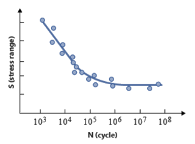
requires a larger certainty of survival).Figure 2. S-N Curve with Scatter Data
To understand these parameters, let us consider the S-N curve as an example. When S-N
testing data is presented in a log-log plot of alternating nominal stress amplitude
Sa or range SR versus cycles to failure N, the relationship between S and N can be
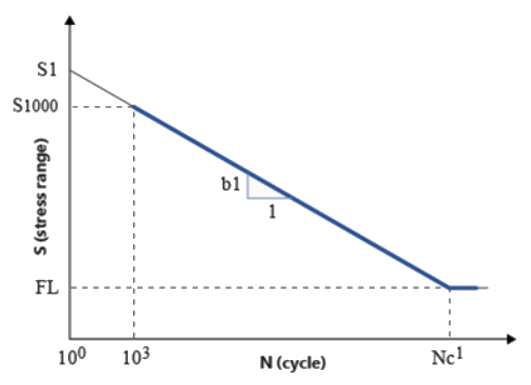
described by straight line segments. Normally, a one or two segment idealization is
used.Figure 3. One Segment S-N Curve in log-log Scale
Consider the situation where S-N scatter leads to variations in the possible S-N
curves for the same material and same sample specimen. Due to natural variations,
the results for full reversed rotating bending tests typically lead to variations in
data points for both Stress Range (S) and Life (N). Looking at the Log scale, there
will be variations in Log(S) and Log(N). Specifically, looking at the variation in
life for the same Stress Range applied, you may see a set of data points which look
like this.
S
2000.0
2000.0
2000.0
2000.0
2000.0
2000.0
Log (S)
3.3
3.3
3.3
3.3
3.3
3.3
Log (N)
3.9
3.7
3.75
3.79
3.87
3.9
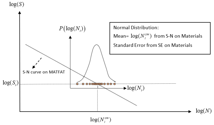
As with many processes, the distribution of Log(N) is assumed to be a Normal
Distribution. There is a full population of possible values of log(N) for a
particular value of log(S). The mean of this full population set is the true
population mean and is unknown. Therefore, statistically estimate the worst true
population mean of log(N) based on the input sample mean SN
curve in Materials and Standard Error in the Material DB and
My Material tabs of the sample. The SN material data input in the
Material DB and My Material tabs is based on the mean of the normal
distribution of the scatter in the particular user sample used to generate the
data.Figure 4. Probability Function of the Log(N) Normal Distribution for
S-N Scatter. of a particular user-defined sample data
The experimental scatter exists in both Stress Range and Life data. In the
Assign Material dialog, the Standard Error of the scatter of log(N) is
required as input (SE field for S-N curve). The sample mean is
provided by the S-N curve as , whereas, the standard error is input via the
SE field in the
Assign Material dialog.
If the specified S-N curve is directly utilized, without any perturbation, the sample
mean is directly used, leading to a certainty of survival of 50%. This implies that
OptiStruct does not perturb the sample mean provided
in the Assign Material dialog. Since a value of 50% survival certainty may
not be sufficient for all applications, HyperLife can internally
perturb the S-N material data to the required certainty of survival defined by you.
To accomplish this, the following data is required.
Standard Error of log(N) normal distribution (SEin
Assign Material).
Certainty of Survival required for this analysis (Certainty of Survival in the Fatigue Module context).
A normal distribution or gaussian distribution is a probability density function
which implies that the total area under the curve is always equal to 1.0.
The user-defined SN curve data is assumed as a normal distribution, which is
typically characterized by the following Probability Density
Function:
Where,
The data value () in the sample.
The sample mean .
The standard deviation of the sample (which is unknown, as you input
only Standard Error (SE) in the Assign Material dialog).
The above distribution is the distribution of the user-defined sample, and not the
full population space. Since the true population mean is unknown, the estimated
range of the true population mean from the sample mean and the sample SE and
subsequently use the user-defined Certainty of Survival to perturb the sample mean.
Standard Error is the standard deviation of the normal distribution created by all
the sample means of samples drawn from the full population. From a single sample
distribution data, the Standard Error is typically estimated as , where is the standard deviation of the sample, and is the number of data values in the sample. The mean
of this distribution of all the sample means is actually the same as the true
population mean. The certainty of survival is applied on this distribution of all
the sample means.
The general practice is to convert a normal distribution function into a standard
normal distribution curve (which is a normal distribution with mean=0.0 and standard
error=1.0). This allows us to directly use the certainty of survival values via
Z-tables.
Note: The certainty of survival is equal to the area of the curve under
a probability density function between the required sample points of interest.
It is possible to calculate the area of the normal distribution curve directly
(without transformation to standard normal curve), however, this is
computationally intensive compared to a standard lookup Z-table. Therefore, the
generally utilized procedure is to first convert the current normal distribution
to a standard normal distribution and then use Z-tables to parameterize the
input survival certainty.
For the normal distribution of all the sample means, the mean of this distribution is
the same as the true population mean , the range of which is what you want to estimate.
Statistically, you can estimate the range of true population mean as:
That is,
Since the value on the left hand side is more conservative, use the following
equation to perturb the SN curve:
Where,
Perturbed value
User-defined sample mean (SN curve on Materials)
Standard error (SE on Materials)
The value of is procured from the standard normal distribution
Z-tables based on the input value of the certainty of survival. Some typical values
of Z for the corresponding certainty of survival values are:
Z-Values (Calculated)
Certainty of Survival (Input)
0.0
50.0
0.5
69.0
1.0
84.0
1.5
93.0
2.0
97.7
3.0
99.9
Based on the above example (S-N), you can see how the S-N curve is modified to the
required certainty of survival and standard error input. This technique allows you
to handle Fatigue material data scatter using statistical methods and predict data
for the required survival probability values.
Adjustment of Single SN Curves
This section describes how a slope-based SN curve is modified in HyperLife.
Certainty of Survival
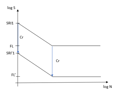
If the certainty of survival is not 0.5 and standard error (SE) is not
0.0, an SN curve is modified by shifting SRI1 and FL.Figure 5.
Where z is a z-value in standard normal distribution that corresponds to
the certainty of survival.
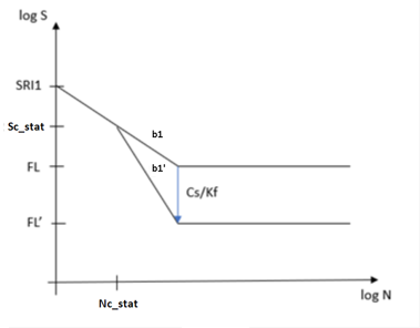
Surface Condition and Fatigue Strength Reduction Factor
A factor for surface condition (Cs) and fatigue strength reduction
factor (Kf) are applied to fatigue limit to modify slope of the SN curve
after Nc_stat cycles in the following manner.
Where Nc_stat is the number of cycles at static failure transition.Figure 6.
Static Failure
When a specimen fails at less than or equal to a certain low number of
cycles, the failure is not considered as a fatigue failure but
considered as a static failure. Once the failure is considered as a
static failure, the low number of cycles is defined as the number of
static failure transition cycles (Nc_stat). In fatigue analysis, stress
amplitudes are supposed to be less than the stress amplitude (Sc_stat)
corresponding to Nc_stat in an SN curve in order to apply fatigue
failure theories. If static failure check is enabled, HyperLife checks
whether stress or stress amplitudes in stress history is greater than
Sc_stat, and reports a warning when a stress or stress amplitude exceeds
Sc_stat.
Nc_stat can be specified in Static Failure options of My
Material.
Sc_stat is defined via alpha in Static Failure options of My
Material, which is a scaling factor to the UTS to determine the
static failure stress threshold.
Database materials are to be saved to My Material to edit the static
failure options.
SN Curve Modification and Static Failure Transition
HyperLife modifies the user-defined SN curve when certainty of survival
is not 0.5, surface treatment is applied, surface finish is applied, or
fatigue strength factor is applied. In the modification due to surface
treatment (Cr), surface finish (Cs), or fatigue strength factor (Kf), SN
curve is only modified after Nc_stat because surface treatment, surface
finish, or fatigue strength factor should not affect static failure
behavior which does not follow fatigue theories.
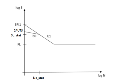
Once static failure check is enabled, HyperLife modifies slope (b0) near
UTS so that number of cycles at UTS can be 1 as depicted in Figure
7. By default, in HyperLife static failure check is set to No
Check (Advance options > Result > Static Failure Check > No Check), with static failure check is disabled, slope near UTS
in SN curve is not modified. HyperLife checks static failure and
continues to evaluate damages of remaining stress history with Continue (Advance options > Result > Static Failure Check > Continue). You can choose an option to stop damage calculation as
soon as OptiStruct detects static failure (Advance options > Result > Static Failure Check > Stop). Depending on the UTS value, there can be a special case
where the calculated slope b0 becomes 0.0. In this case damage is 1.0
for all the stress amplitudes greater than or equal to Sc_stat. Figure 7.
Instead of HyperLife calculating b0 using UTS and Sc_stat, you can
define b0 directly in Static Failure options
in MyMaterial. If b0 is defined, b0 is honored as it is. If b0 is
set to 0.0, damage at Sc_stat is 1.0, and damage at stress amplitude
greater than Sc_stat is more than 1.0.
You can choose how Nc_stat
is defined in Static Failure options. You can
directly define Nc_stat. This is the default way to define Nc_stat. The
default value of Nc_stat is 1000. Another way to define Nc_stat is to
specify Sc_stat. Sc_stat is specified by a fraction of UTS (using alpha
field in Static Failure options). Default Sc_stat value is 0.9*UTS. If
Sc_stat is specified, HyperLife calculates Nc_stat using the slope of
the SN curve after SN curve shift due to certainty of survival.
If static failure check is activated, static failure is reported when
the maximum stress is higher than Sc_stat or corrected stress range is
more than Sc_stat.
If static failure check (Continue in Static
Failure options) is set, the SN curve is modified so that HyperLife can
report a damage value of 1.0 when stress range is 2*UTS and 2*UTS is
smaller than SRI1. Thus, stress range higher than Sc_stat reports a
damage value different from the user-defined SN curve due to the
modified b0 slope in the picture. If static failure check is set to
STOP, damage is greater than 1 when stress range is more than Sc_stat.
HyperLife stops the run if 2*UTS is less than Sc_stat.
Note:Advance options > Result > Static Failure Transition Cycle > Life/Stress defines which option should drive the static failure
check.
Static Failure Transition Cycle = Stress
The option defines stress amplitude threshold with alpha*UTS in static
failure options in MyMaterial.
A cycle corresponding to the threshold amplitude is the static failure
transition cycle Nc_stat. If static failure check is not “no check”, SN
slope at static failure region (b0) is determined by UTS and alpha*UTS
unless user defines b0. If internally calculated b0 is 0.0, damage of
stress amplitude higher than or equal to alpha*UTS is 1.0.
Static Failure Transition Cycle = Life (default)
The option directly defines transition cycle with Nc_stat in static
failure options in MyMaterial. If static failure check is not “no
check”, the following statements apply to SN curve: SN slope at static
failure region is determined by UTS and Stress amplitude corresponding
to Nc_stat by default. if b0 is defined by user in MATFAT, the b0 will
be used for the SN slope at static failure region . If b0 =0.0, damage
value is 1 at life = Nc_stat, and damage for life shorter than Nc_stat
is greater than 1.
Overall SN Curve Modification
Figure 8. Combining factors from certainty of survival, surface condition,
fatigue strength reduction factor, and static failure, the final SN
curve that is used in damage calculation is depicted in Figure 8.
Adjustment of Multiple SN Curves
The following adjustment is applied to multi-mean stress SN curves, multi-stress
ratio SN curves and Haigh diagram.
Certainty of Survival
Uncertainty of fatigue strength of material can be taken into
consideration by means of the standard error of log(stress) and
certainty of survival.
For example, if the standard error of log(stress) is 0.2, and certainty
of survival has to be 99.7%, HyperLife
adjusts the multiple SN curves as follows:
log(fatigue strength) = log(user defined fatigue strength) – 3 x
0.2
Fatigue strength = (user defined fatigue strength ) x 10(-3 x
0.2) .
In the example, user defined fatigue strength is reduced by 3 standard
error which corresponds to 99.7% in normalized Gaussian
distribution.
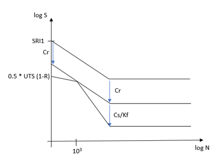
Surface Condition and Fatigue Strength Reduction Factor
A factor for surface condition (Cs) and fatigue strength reduction
factor (Kf) are applied to fatigue strength in the following
manner:
Fatigue strength = (user defined fatigue strength ) * K’
Where,
K’ = 1.0 for N <= 1000
K’ = Cs/Kf for N >
Nc1
log(K’) = log(Cs/Kf) x (3-logN) / (3-logNc1) for 1000 <
N < Nc1
Nc1 : transition point
Standard Error of Cyclic Stress-Strain in Strain Life
The Standard Error of Cyclic Stress-Strain curve is defined via the SEc field for EN
fatigue. The value of SEc is used to modify the cyclic strength coefficient
as:
Where,
K' = Cyclic strength coefficient.
n' = Strain Cyclic hardening exponent.
z = value of normal distribution calculated using the certainty of survival.
SEc is input via the Strain Life material properties in My Material Context.
References
1 Yung-Li Lee, Jwo. Pan, Richard B. Hathaway and Mark E.
Barekey. Fatigue testing and analysis: Theory and practice, Elsevier,
2005