Random Response Fatigue Analysis

The study of fatigue life of structures under Random Loading.

Power Spectral Density (PSD) results from the Random Response Analysis are used to calculate Moments ( $m_{n}$ ) that are used to generate the probability density function for the number of cycles versus the stress range.

There are two ways to perform Random Response Fatigue Analysis in HyperLife:

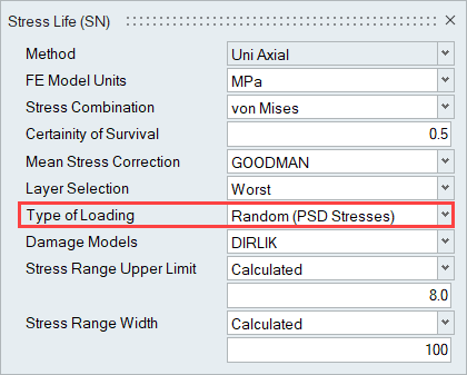
by using PSD Stresses which are already available for Random Fatigue
by using PSD Stresses generated from Frequency Response Analysis and Power Spectral Density Functions Loading versus Frequency in HyperLife

PSD Stresses Are Already Available for Random Fatigue

The PSD Moments are calculated based on the Stress PSD generated from the Random Response Analysis, as shown below.

Input

Calculates Random Response Fatigue.

Power Spectral Density (PSD) Moments

PSD Moments (

m_{n}

) are calculated based on the Stress PSD generated from the Random Response Analysis as:

Figure 1. Calculation of PSD Moments

The moments are calculated based on:(1)

m_{n} = \sum_{k = 1}^{N} f_{k}^{n} G_{k} δ f

Where,

$f_{k}$: Frequency value
$G_{k}$: PSD response value at frequency $f_{k}$

The stability of $m_{0}$ can be checked by setting PARAM, CHKM0, YES. A warning is printed if the frequency interval must be further refined.

Calculate Probability of Stress Range Occurrence

Calculation of the Probability of occurrence of a stress range between the initial and final stress range values within each bin section are user-defined.

The probability $P (Δ S_{i})$ of a stress range occuring between $(Δ S_{i} - δ S / 2)$ and $(Δ S_{i} + δ S / 2)$ is $P (Δ S_{i}) = p_{i} δ S$ .

Probability Density Function (probability density of number of cycles versus stress range)

PSD Moments calculated as shown above are used in the generation of a Probability Density Function $f (m_{n})$ for the stress range. The function is based on the specified damage model in the Random Response Fatigue section of the SN Fatigue module. Currently, DIRLIK, LALANNE, NARROW, and THREE options are available to define the damage model.

DIRLIK (Default Damage Model):

DIRLIK postulated a closed form solution to the determination of the Probability Density Function as:(2)

p (S) = \frac{\frac{D_{1}}{Q} e^{\frac{- Z}{Q}} + \frac{D_{2} Z}{R^{2}} e^{\frac{- Z^{2}}{2 R^{2}}} + D_{3} Z e^{\frac{- Z^{2}}{2}}}{2 \sqrt{m_{0}}}

Where,

$D_{1} = \frac{2 (x_{m} - γ^{2})}{1 + γ^{2}}$
$D_{2} = \frac{1 - γ - D_{1} + D_{1}^{2}}{1 - R}$
$D_{3} = 1 - D_{1} - D_{2}$
$Z = \frac{S}{2 \sqrt{m_{0}}}$
$Q = \frac{1.25 (γ - D_{3} - D_{2} R)}{D_{1}}$
$R = \frac{γ - x_{m} - D_{1}^{2}}{1 - γ - D_{1} + D_{1}^{2}}$
$γ = \frac{m_{2}}{\sqrt{m_{0} m_{4}}}$: Irregularity Factor
$x_{m} = \frac{m_{1}}{m_{0}} \sqrt{\frac{m_{2}}{m_{4}}}$
$S$: Stress range

LALANNE:

The LALANNE Random Fatigue Damage model depicts the probability density function as: (3)

p (S) = \frac{1}{2 \sqrt{m_{0}}} (\frac{\sqrt{1 - γ^{2}}}{\sqrt{2 π}} e^{\frac{- S^{2}}{8 m_{0} (1 - γ^{2})}} + \frac{S γ}{4 \sqrt{m_{0}}} e^{\frac{- S^{2}}{8 m_{0}}} (1 + E r f (\frac{S γ}{2 \sqrt{2 m_{0} (1 - γ^{2})}})))

Where,

$γ = \frac{m_{2}}{\sqrt{m_{0} m_{4}}}$: Irregularity factor
$S$: Stress range

NARROW:

The Narrow Band Random Fatigue Damage model uses the following probability functions:(4)

p (S) = (\frac{S}{4 m_{0}} e^{- (\frac{S^{2}}{8 m_{0}})})

Where, $S$ is the stress range.

In the NARROW band model, by default, HyperLife uses number of zero crossings ( $n_{z c r o s s} = \sqrt{m_{2} / m_{0}}$ ) instead of number of peaks ( $n_{p e a k s} = \sqrt{m_{4} / m_{2}}$ ), because the numerical calculations involving $m_{4}$ may lead to unstable numerical behavior.

THREE:

The Steinberg 3-Band Random Fatigue Damage model uses the following probability function.

Unlike the other damage models, for THREE band, the following values are probability (and not probability density). This is also evident in the use of upper case

P (S)

compared to the lower case

p (S)

for the other damage models. For the THREE damage model, the following probabilities are directly used to calculate the number of cycles by multiplying

P (S)

with the total number of zero-crossings in the entire time history (for other damage models (except THREE), the probability density values are first multiplied by DS (bin size) to get the probability).(5)

P (S) = {\begin{matrix} 0.683 at 2 \sqrt{m_{0}} \\ 0.271 at 4 \sqrt{m_{0}} \\ 0.043 at 6 \sqrt{m_{0}} \end{matrix}

Where, $S$ is the stress range.

Figure 2. Probability Density Function (probability density of number of cycles versus stress range)

The probability density function can be adjusted based on the following parameters defined in the Random Response Fatigue section of the SN Fatigue module:

Upper Stress Range (Calculated): Calculates the upper limit of the stress range. This is calculated as: upper limit of the stress range = 2*RMS Stress*Upper Stress Range (Calculated) input. The RMS Stress is output from Random Response Subcase. The stress ranges of interest are limited by the upper limit of the stress range. Any stresses beyond the upper limit are not considered in Random Fatigue Damage calculations.
Width: Stress Range (Calculated): Calculates the width of the stress ranges (DS = $δ S$ ) for which the probability is calculated (Figure 2). The default is 100 and the first bin starts from 0.0 to $δ S$ . The width of the stress range is calculated as DS = upper limit of the stress range / Width: Stress Range (Calculated).

Calculate Probability of Stress Range Occurrence

Calculation of the Probability of occurrence of a stress range between the initial and final stress range values within each bin section are based on the damage models.

DIRLIK, LALANNE, and NARROW Damage Models

The probability $P (S_{i})$ of a stress range occurring between $(S_{i} - δ S / 2)$ and $(S_{i} + δ S / 2)$ is $P (S_{i}) = p_{i} (S_{i}) δ S$ .

THREE Damage Model

The probability is directly defined using the probability function defined above. It is being repeated here for clarity.(6)

P (S) = {\begin{matrix} 0.683 at 2 \sqrt{m_{0}} \\ 0.271 at 4 \sqrt{m_{0}} \\ 0.043 at 6 \sqrt{m_{0}} \end{matrix}

Where, $S$ is stress range.

For the THREE damage model, there are only three bins. The number of cycles at each stress range (2*RMS, 4*RMS, and 6*RMS) are calculated by directly multiplying the corresponding probabilities with the total number of zero-crossings (refer to section below regarding calculation of number of zero-crossings).

Select Damage Models

DIRLIK, LALANNE, NARROW, and THREE are available for selection in the Random Response Fatigue section of the SN Fatigue module. The following information may provide additional understanding to help choose the damage model for a HyperLife run.

You can see from the previous sections, that the PSD moments of stress are used to calculated corresponding moments, which are used to determine the probability density function for the stress-range.
DIRLIK and LALANNE models generate probabilities across a wider distribution of the stress-range spectrum. Therefore, these models should be used when the input random signal consists of a variety of stress-ranges across multiple frequencies. Therefore, the information in the probability density function better captures the wider range in stress-range distribution if DIRLIK and LALANNE are used.
The NARROW model is intended for random signals for which the stress range is expected to be closely associated with a high probability of particular certain stress range distribution. Therefore, if you know that the input random data does not have a wide range of stress-range distribution, and that the distribution is mainly concentrated about a particular stress range, then you should select NARROW, since it expects the highest probability of stress-ranges to lie at or around this particular stress range.
The THREE model is like the NARROW model, except that it expects the distribution of the random signal to contain, in addition to the association with 1*RMS, associations (albeit smaller) with 2*RMS, and 3*RMS. Therefore, if your input random data is mainly clustered around stress ranges in 1*RMS, and to a lesser extent, 2*RMS, and 3*RMS, then you should select THREE.

Number of Peaks and Zero Crossings

NARROW and THREE Damage Models

The number of zero crossings per second in the original time-domain random loading (from which the Frequency based Random PSD load is generated) is determined as:(7)

n_{z c r o s s} = \sqrt{\frac{m_{2}}{m_{0}}}

DIRLIK and LALANNE Damage Models

The number of peaks per second in the original time-domain random loading (from which the Frequency based Random PSD load is generated) is determined as:(8)

n_{p e a k s} = \sqrt{\frac{m_{4}}{m_{2}}}

Where, $m_{n}$ is the corresponding moments calculated, as shown in Power Spectral Density (PSD) Moments.

The total number of cycles for THREE band and NARROW band is calculated as:(9)

N_{T} = n_{z c r o s s} T

The total number of cycles for DIRLIK, LALANNE, and NARROW is calculated as:(10)

N_{T} = n_{p e a k s} T

Where, $T$ is Total exposure time given by the Repeats/Time values when creating events in the Load Map dialog.

Total Number of Cycles of a Particular Stress Range

The total number of cycles with Stress range

Δ S_{i}

is calculated as:(11)

N_{i} = P (S_{i}) N_{T}

Fatigue Life and Damage

Fatigue Life (maximum number of cycles of a particular stress range

S_{i}

for the material prior to failure) is calculated based on the Material SN curve as:(12)

N_{f} (S_{i}) = {(\frac{S_{i}}{S_{f}})}^{\frac{1}{b}}

Total Fatigue Damage as a result of the applied Random Loading is calculated based on:(13)

D = \sum_{i = 1}^{N} \frac{N_{i}}{N_{f} (S_{i})}

To account for the mean stress correction with any loading that leads to a mean stress different from zero, you can define a static subcase that consists of such loading (typically gravity loads). This static subcase can be referenced within the fatigue event created in the Load Map dialog.

Setup

After loading an FE result file that contains a Random subcase, Random Response Fatigue is activated by setting the Type of Loading field to Random (PSD Stresses). The supported result datatypes for Random Fatigue are Segalman Von mises PSD stresses (Stress Life only) or Absolute Max Principal PSD Stresses (Stress Life and Strain Life).

PSD Stresses to be Generated from Frequency Response Analysis and Power Spectral Density Functions Loading vs Frequency in HyperLife for Random Fatigue

The PSD stresses are calculated internally using the FRF stresses and the input PSDs. The fatigue event created first calculates the PSD stress (Random Response Analysis), which are then used to calculate the PSD moments.

Different Load Cases (a and b)

H_{x a} (f)

and

H_{x b} (f)

are the complex frequency responses (stresses) of the

x

^th degree of freedom, due to Frequency Response Analysis load cases

a

and

b

respectively, the power spectral density of the response of the

x

^th degree of freedom,

S_{x o} (f)

is:(14)

S_{x o} (f) = H_{x a} (f) S_{a b} (f) H_{x b} (f)

Where, $S_{a b} (f)$ is the cross power spectral density of two (different, $a \neq b$ ) sources, where the individual source $a$ is the excited load case and $b$ is the applied load case. This value can possibly be a complex number.

Same Load Case (a)

S_{a} (f)

is the spectral density of the individual source (load case

a

), the power spectral density of the response of

x

^th degree of freedom due to the load case

a

will be:(15)

S_{x o} (f) = {| H_{x a} (f) |}^{2} S_{a} (f)

Combination of Different (a,b) and Same (a,a) Load Cases in a Single Random Response Analysis

If there is a combination of load cases for Random Response Analysis, the total power spectral density of the response will be the summation of the power spectral density of responses due to all individual (same) load cases as well as all cross (different) load cases.

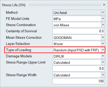
Setup

After loading an FE result file that contains a Frequency Response Analysis subcase, Random Response Fatigue is activated by setting the Type of Loading field to Random (Input PSD with FRF).

If the power spectral density of the loading versus frequency is of Magnitude and Phase, it is converted to real and imaginary.

Loadmap:

Input PSD is based on the Channel Type selection.

Input PSD: Real and Imaginary
Input PSD: Magnitude and Phase

The event is created with the correlations based on the number of Frequency Response Subcases selected. The imported channels (input power spectral density of the Loading vs Frequency) are then assigned to each correlation.

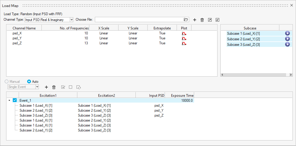
Excitation1 and Excitation2 refer to the correlations of the FRF subcases. The Input PSDs are used to scale the complex stresses. If the Input PSDs are of the Phase and Magnitude form, they are internally converted to Real and Imaginary.

PSD Stresses calculated from the above event are then utilized for fatigue calculations, like the case where PSD stresses are already available (described in the beginning of this chapter).

Note: RMS stress value over the entire frequency range is output along with damage and life.